
There are two types of streaming processing modes, Stateless and Stateful. Stateless is easy to understand that each message is processed independently without the needs to maintain the states across multiple messages. The challenge and fun one is the Stateful streaming processing where the processing of a message depends on the result of the processing of previous messages. From this blog post, I will look into how stateful operations work on Spark Structured Streaming. In this blog post, I first discuss the state management in Spark Structured Streaming and then explore how limit, deduplicate, and aggregate operators work under the hood. I will cover the session window aggregation, streaming-streaming join, and arbitrary stateful operations in the next few blog posts.
State Management
While processing stateful operations, the processing of current message depends on the result from the processing of the previous messages. To achieve that, the result of the processing of previous messages, i.e., the current state of the streaming operation, needs to be read by the current processing session, and the result of the processing of the current message, i.e., the updated state of the streaming operation, needs to be stored somewhere for future access.
Spark Structured Streaming uses State Stores to maintain the states of the stateful operations in streaming queries. A State Store is a key-value store where the stateful operators can read and write state record. Spark Structured Streaming provides the StateStoreRDD and ReadStateStoreRDD that is the abstract representation of the state store operations.
A stateful operator defines its StateStoreRDD instance through the mapPartitionsWithStateStore and the mapPartitionsWithReadStateStore methods of the StateStoreOps implicit class. The stateful operator defines the operation logics, including the state store read and write operations, in an anonymous function and pass it into the mapPartitionsWithStateStore method and the mapPartitionsWithReadStateStore method. The mapParitionsWithStateStore creates the StateStoreRDD for updating the state stores, which get or create the state store instance for each partition in executors and call the anonymous function with the state store. The mapPartitionsWithReadStateStore method does the similar things but creates the ReadStateStoreRDD for read-only operations of the state stores.

The partitions of a StateStoreRDD (and the ReadStateStoreRDD) are same as the data RDD which the stateful operator works on. There is a 1:1 mapping between a data partition and a StateStoreId. A StateStoreId uniquely identify a state store, consisting of (checkpointRootLocation, operatorId, partitionId, and storeName). A state store maintains the versioned key-value pairs, each version of the data representing the operation state at a specific point. The StateStore class encapsulates the methods for accessing a state store. Each instance of a StateStore represents a specific version of stat data, and such instances are created by their respective StateStoreProvider.
For each unique state store, a StateStoreProvider instance is created in an executor when the first batch of streaming query is executed on this executor and the subsequent batches reuse this provider to fetch the StateStore instance. The StateStoreProvider exposes with a getStore(version: Long) method to return an instance of the StateStore representing state data of the given version. The StateStoreProvider also exposes a getReadStore(version: Long) method that returns an instance of ReadStateStore class. At the core, a ReadStateStore instance is same as the StateStore instance returned by the getStore method but wrapped to prevent modification.
Up to Spark v3.3, there are two built-in implementations of StateStoreProvider, HDFSBackedStateStoreProvider and RocksDBStateStoreProvider. HDFSBackedStateStoreProvider maintains the state data at two stages. It uses a Java ConcurrentHashMap to store the state data in memory at first stage and then back up the state data in an HDFS-compatible file system at the second stage. HDFSBackedStateStoreProvider is the default implementation of StateStoreProvider. RocksDBStateStoreProvider is a new feature released in Spark v3.2. RocksDBStateStoreProvider is introduced to handle the streaming queries that involve a large volume of state data which cause heavy JVM GC loads. The RocksDBStateStoreProvider takes advantage of the RocksDB for optimised state management in the native memory and the local disk, instead of using the JVM memory as the HDFSBackedStateStoreProvider does.

From the previous blog post that discusses the Azure Event Hub integration, Spark Structured Streaming Deep Dive (4) – Azure Event Hub Integration, we learnt the benefits of locality of event hub connections and receivers where some partition is allocated to the same executors across all batches so that event hub connection and receiver instances can be cached and reused across batches, instead of having to create and initialise during each batch execution. For state management in executors, we want to cache and reuse the StateStoreProviders in the same executor across batches as well. It can be expensive to change the location of state store providers that involves the extra overhead of loading checkpointed states.
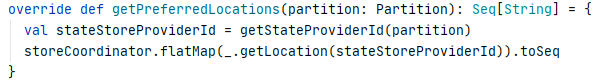
Spark Structured Streaming comes with the StateStoreCoordinator for coordinating the state store providers across the executors in the cluster. The StateStoreCoordinator instance is running on the Driver, with a hash map holding the executor location where each state store providers is actively running. In the StateStoreRDD, the getPreferredLocations method calls the StateStoreCoordinator to get the executor that has the StateStoreProvider instance loaded for a partition and set the preferred location of this partition to that executor.
Each StateStore instance running on an executor holds a StateStoreCoordinatorRef that reference to the StateStoreCoordinator instance running on the driver. The StateStore instance can communicate with the StateStoreCoordinator through the StateStoreCoordinatorRef for reporting active state store provider instance or verify whether an executor has the active instance of a state store.
In the rest of the blog post, I will walk through how Limit, Duplicate and Aggregate stateful operators work.
Limit
Firstly, let’s have a look at a streaming query example that involves a Limit operation and the execution plan of the query.

The streaming query is very simple with only one limit operation to return only 5 items from the data stream.
Here is the execution plan of this streaming query.
== Parsed Logical Plan ==
GlobalLimit 5
+- LocalLimit 5
   +- StreamingRelationV2 org.apache.spark.sql.execution.streaming.sources.RateStreamProvider@54348ac, rate, org.apache.spark.sql.execution.streaming.sources.RateStreamTable@38152b21, [rowsPerSecond=3], [timestamp#95880, value#95881L]

== Analyzed Logical Plan ==
timestamp: timestamp, value: bigint
GlobalLimit 5
+- LocalLimit 5
   +- StreamingRelationV2 org.apache.spark.sql.execution.streaming.sources.RateStreamProvider@54348ac, rate, org.apache.spark.sql.execution.streaming.sources.RateStreamTable@38152b21, [rowsPerSecond=3], [timestamp#95880, value#95881L]

== Optimized Logical Plan ==
GlobalLimit 5
+- LocalLimit 5
   +- StreamingRelationV2 org.apache.spark.sql.execution.streaming.sources.RateStreamProvider@54348ac, rate, org.apache.spark.sql.execution.streaming.sources.RateStreamTable@38152b21, [rowsPerSecond=3], [timestamp#95880, value#95881L]

== Physical Plan ==
StreamingGlobalLimit 5, state info [ checkpoint = <unknown>, runId = 739e70b3-8649-466d-8497-695d8bd5abe1, opId = 0, ver = 0, numPartitions = 200], Append
+- Exchange SinglePartition, ENSURE_REQUIREMENTS, [id=#13150]
   +- *(1) LocalLimit 5
      +- StreamingRelation rate, [timestamp#95880, value#95881L]
From the execution plan we can see the query reads data from a Rate stream source which generate 3 random number every second. The query first executes a LocalLimit operation and then a GlobalLimit operation on the result of the LocalLimit operation. This aligns with the rule defined in the StreaminGlobalLimitStrategy that first plans a StreamingLocalLimitExec and then uses it as child to plan the StreamingGlobalLimitExec.

Internally, the StreamingLocalLimitExec operator executes the limit operation locally on each partition of a micro-batch, i.e., takes 5 items for each partition in our query example. For example, if there are 10 partitions, there will be 10 x 5 = 50 items taken in total. The StreamingGlobalLimitExec operator executes the limit operation on the results from all partitions. As the requiredChildDistribution of StreamingGlobalLimitExec operator is “AllTuples” (i.e., single partition), an Exchange operation is first executed to have all the 50 items from the 10 partitions clustered in a single partition, and then the StreamingGlobalLimitExec operator is executed that first reads the total row count taken from previous micro-batches from the state store, and then takes items from the current micro-batch and adds the row count to the cumulative total row count. If the total row count is over the limit, the remaining items will not be returned. When the current micro-batch is completed, the updated total row count is written back to the state store.

Deduplicate
Again, example and execution plan first.

In this stream query, the rows with “key” value being same as an existing row will be dropped.
Here is the execution plan of the query.
== Parsed Logical Plan ==
Deduplicate [key#36171L]
+- Project [timestamp#36167, value#36168L, CEIL((rand(-8825895992041344291) * cast(10 as double))) AS key#36171L]
   +- StreamingRelationV2 org.apache.spark.sql.execution.streaming.sources.RateStreamProvider@2b7cf98f, rate, org.apache.spark.sql.execution.streaming.sources.RateStreamTable@25bb1290, [rowsPerSecond=3], [timestamp#36167, value#36168L]

== Analyzed Logical Plan ==
timestamp: timestamp, value: bigint, key: bigint
Deduplicate [key#36171L]
+- Project [timestamp#36167, value#36168L, CEIL((rand(-8825895992041344291) * cast(10 as double))) AS key#36171L]
   +- StreamingRelationV2 org.apache.spark.sql.execution.streaming.sources.RateStreamProvider@2b7cf98f, rate, org.apache.spark.sql.execution.streaming.sources.RateStreamTable@25bb1290, [rowsPerSecond=3], [timestamp#36167, value#36168L]

== Optimized Logical Plan ==
Deduplicate [key#36171L]
+- Project [timestamp#36167, value#36168L, CEIL((rand(4175393523432276970) * 10.0)) AS key#36171L]
   +- StreamingRelationV2 org.apache.spark.sql.execution.streaming.sources.RateStreamProvider@2b7cf98f, rate, org.apache.spark.sql.execution.streaming.sources.RateStreamTable@25bb1290, [rowsPerSecond=3], [timestamp#36167, value#36168L]

== Physical Plan ==
StreamingDeduplicate [key#36171L], state info [ checkpoint = <unknown>, runId = ca626e17-d266-4ad9-9301-a6b75fdfe1a0, opId = 0, ver = 0, numPartitions = 200], 0
+- Exchange hashpartitioning(key#36171L, 200), ENSURE_REQUIREMENTS, [id=#9514]
   +- *(1) Project [timestamp#36167, value#36168L, CEIL((rand(4175393523432276970) * 10.0)) AS key#36171L]
      +- StreamingRelation rate, [timestamp#36167, value#36168L]
From the execution plan, we can see that the data is reshuffled to have the rows with the same “key” located at the same partition. Then the StreamingDeduplicateExec operator is executed. The execution of the StreamingDeduplicateExec operator is pretty simple. For each partition, the operator first retrieves the state record for the same “key” from the state store. If there is a state record for this “key”, that implies a record with the same “key” has been processed by the previous micro-batch or by the previous action in the same micro-batch. If so, this record is not returned. If there is no record with the same “key” in the state store, this record will be returned and the “key” of the record will be written into the state store.

Aggregate
Once again, example and execution plan first.

In this example, the incoming streaming data is grouped by “key” column and row count for each “key” group is calculated.
== Parsed Logical Plan ==
'Aggregate ['key], ['key, count(1) AS count#30789L]
+- Project [timestamp#30777, value#30778L, CEIL((rand(-7074935109240296984) * cast(10 as double))) AS key#30781L]
   +- StreamingRelationV2 org.apache.spark.sql.execution.streaming.sources.RateStreamProvider@42dfa827, rate, org.apache.spark.sql.execution.streaming.sources.RateStreamTable@2cffd62d, [rowsPerSecond=3], [timestamp#30777, value#30778L]

== Analyzed Logical Plan ==
key: bigint, count: bigint
Aggregate [key#30781L], [key#30781L, count(1) AS count#30789L]
+- Project [timestamp#30777, value#30778L, CEIL((rand(-7074935109240296984) * cast(10 as double))) AS key#30781L]
   +- StreamingRelationV2 org.apache.spark.sql.execution.streaming.sources.RateStreamProvider@42dfa827, rate, org.apache.spark.sql.execution.streaming.sources.RateStreamTable@2cffd62d, [rowsPerSecond=3], [timestamp#30777, value#30778L]

== Optimized Logical Plan ==
Aggregate [key#30781L], [key#30781L, count(1) AS count#30789L]
+- Project [CEIL((rand(-8495241975996027045) * 10.0)) AS key#30781L]
   +- StreamingRelationV2 org.apache.spark.sql.execution.streaming.sources.RateStreamProvider@42dfa827, rate, org.apache.spark.sql.execution.streaming.sources.RateStreamTable@2cffd62d, [rowsPerSecond=3], [timestamp#30777, value#30778L]

== Physical Plan ==
*(4) HashAggregate(keys=[key#30781L], functions=[finalmerge_count(merge count#30793L) AS count(1)#30788L], output=[key#30781L, count#30789L])
+- StateStoreSave [key#30781L], state info [ checkpoint = <unknown>, runId = 05909616-8b27-4e84-a5c0-32ec697cfeaa, opId = 0, ver = 0, numPartitions = 200], Append, 0, 2
   +- *(3) HashAggregate(keys=[key#30781L], functions=[merge_count(merge count#30793L) AS count#30793L], output=[key#30781L, count#30793L])
      +- StateStoreRestore [key#30781L], state info [ checkpoint = <unknown>, runId = 05909616-8b27-4e84-a5c0-32ec697cfeaa, opId = 0, ver = 0, numPartitions = 200], 2
         +- *(2) HashAggregate(keys=[key#30781L], functions=[merge_count(merge count#30793L) AS count#30793L], output=[key#30781L, count#30793L])
            +- Exchange hashpartitioning(key#30781L, 200), ENSURE_REQUIREMENTS, [id=#5433]
               +- *(1) HashAggregate(keys=[key#30781L], functions=[partial_count(1) AS count#30793L], output=[key#30781L, count#30793L])
                  +- *(1) Project [CEIL((rand(-8495241975996027045) * 10.0)) AS key#30781L]
                     +- StreamingRelation rate, [timestamp#30777, value#30778L]
From the execution plan, we can see that the streaming aggregate operation uses the same hash aggregate operators as those used in batch queries. You can find more details of the aggregate operators in my previous blog posts:
- Spark SQL Query Engine Deep Dive (8) – Aggregation Strategy
- Spark SQL Query Engine Deep Dive (9) – SortAggregateExec
- Spark SQL Query Engine Deep Dive (10) – HashAggregateExec & ObjectHashAggregateExec
The main differences are the additional StateStoreRestore, StateStoreSave operations and the extra aggregate operations on the state data.
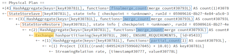
In short, a partial aggregation by grouping key is conducted inner each partition, following by an exchange operation for shuffling data with the same key into a same partition. A partial merge aggregation is then conducted by grouping key on the clustered data to get the aggregation per group at the current micro-batch scope. The StateStoreRestoreExec operator is then executed to get the aggregated value from previous batches. Another partial merge operation is then conducted to aggregate the aggregated value from previous batches from the state store and the aggregated value from the current batch. The updated aggregated value will be written back into the state store by the StateStoreSave operator. Finally, a final aggregate merge operation is conducted to merge the results from all groups.
