In this blog post, I will explain the Dynamic Partition Pruning (DPP), which is a performance optimisation feature introduced in Spark 3.0 along with the Adaptive Query Execution optimisation techniques (which I plan to cover in the next few of the blog posts).

At the core, the Dynamic Partition Pruning is a type of predicate push down optimisation method, which aims to minimise I/O costs of the data read from the data sources. The Dynamic Partition Pruning is especially effective for a common query pattern in BI solutions: a large fact table joins to a number of much smaller dimension tables and the fact table needs to be sliced and diced by some attributes of the dimension tables.

How does the Dynamic Partition Pruning work?

Before diving into the technical details of how the DPP is implemented in Spark, let’s look into the following example to understand how the DPP could improve the query performance.

Here, we have two Spark SQL tables using parquet file formats. The small dimension table, Customers, has the 100 rows with unique customer_id and a grade field with values ranging from 0 to 9.

CREATE TABLE Customers
USING parquet
AS
  SELECT 
    id AS customer_id,
    CAST(rand()*10 AS INT) AS grade
  FROM RANGE(100);

The other table, Orders, is a fact table with 100,000 transactional records. This table has the foreign key, customer_id, to the Customers table. In addition, this table is partitioned by the customer_id, i.e., the orders made by the same customer are stored in the same partition.

CREATE TABLE Orders
USING parquet
PARTITIONED By (customer_id)
AS
  SELECT 
    CAST((rand()*100) AS INT) AS customer_id,
    CAST(rand() * 100 AS INT) AS quantity
FROM RANGE(100000);

Now, we want to run the following query to find all the order records made by customers in grade “5”.

SELECT o.customer_id, o.quantity
FROM Customers AS c
  JOIN orders AS o 
    ON c.customer_id = o.customer_id 
WHERE c.grade =5

Firstly, we run the query with the DPP disabled. From the physical query plan, we can see the query is executed with the “static” optimisations as expected: the small customers table is first filtered by “grade=5” and the filtered customers dataset is broadcasted to the workers to avoid shuffling.

On the large Orders table side, all the 100 partitions of the parquet data source are scanned. 800 data files and 22,236 rows are read from the data source.

Now let’s run the same query with the DPP turned on to see what happens.

set spark.sql.optimizer.dynamicPartitionPruning.enabled = true;

From the physical query plan, we can see that there is not much change on the customers join branch where the customers table is filtered and broadcasted to workers for joining the orders side. However, on the orders join branch, the results of the customers broadcast is reused as the filter criteria pushed down to the parquet data source reader, which only reads the partitions with the partition key (i.e., customer_id in this example) in the broadcast results (i.e., the list of the customers with “grade=5”).

The new query execution logic can also be understood as:

SELECT o.customer_id, o.quantity
FROM Orders o
WHERE o.customer_id IN (
  SELECT customer_id
  FROM Customers
  WHERE grade=5
)

From the data source read statistics, we can see much less data is read from the parquet data files: Only 10 out of the 100 partitions and 80 out of the 800 files are scanned this time. Meantime, we can see one additional metric, “dynamic partition pruning time”, is included which indicates the DPP is applied for this query.

How is the Dynamic Partition Pruning Implemented in Spark SQL?

The Dynamic Partition Pruning feature is implemented in Spark SQL mainly through two rules: a logical plan Optimizer rule, PartitionPruning, and a Spark planner rule, PlanDynamicPruningFilters.

PartitionPruning

The PartitionPruning rule is added to one of the default batches in SparkOptimizer so that it will be applied at the logical plan optimisation stage. The PartitionPruning rule mainly does the following things when it is applied:

1. Check the applicability of the DPP based on the type and selectivity of the join operation
2. Estimate whether the partition pruning will bring benefits or not
3. Insert a DPP predicate, if all the conditions are met

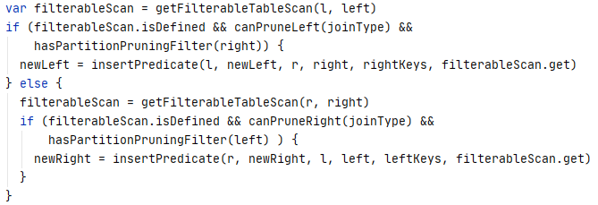
The PartitionPruning rule first checks whether the DPP is applicable or not based on the type and selectivity of the join operation. It starts from checking the applicability of the DPP on the left side of the join. Firstly, the getFilterableTableScan method is used to ensure the left-side table scan can be filtered for a given column. The table scan needs to be either a V1 partitioned scan for a given partition column or a V2 scan which supports runtime filtering on a given attribute. Then the join type is checked by the canPruneLeft method to ensure the join type supports pruning partitions on the left side (the join type needs to be either Inner, LeftSemi, or RightOuter for supporting left side partition pruning). Meantime, the hasPartitionPruningFilter method is used to check whether the right-side of the join has selective predicate which can filter the join key. When all of the above checks are passed, the PartitionPruning rule calls the insertPredicate method to insert predicate on the left side of the join. If no, the same checks are conducted on the right side to evaluate the applicability of the DPP on the right side.

Prior to inserting a DPP predicate, the insertPredicate method runs the pruningHasBenefit method to estimate the costs and benefits of the DPP optimisation and only inserts the DPP predicate when the benefits are bigger than the costs or exchange reuse is enabled for the current Spark session. The pruningHasBenefit method estimates the benefits of the DPP using the size in bytes of the partitioned plan on the pruning side times the filterRatio and estimates the costs of the DPP using the total size in bytes of the other side of the join. The filterRatio is estimated using column statistics if they are available, otherwise using the configured value of spark.sql.optimizer.dynamicPartitionPruning.fallbackFilterRatio.

When the DPP is estimated as beneficial to the query plan or exchange reuse is enabled, a DPP predicate is inserted into the pruning side of the join using the filter on the other side of the join. A custom DynamicPruning expression is created that wraps the filter in an IN expression. Here is the DPP optimised logical plan of the example used above.

PlanDynamicPruningFilters

During the logical plan optimisation stage, the PartitionPruning rule inserts a duplicated subquery with the filter from the other side. The PlanDynamicProuningFilters Spark planner rule is then applied at the execution plan preparation stage, which aims at removing the subquery duplicate by reusing the results of the broadcast.

The PlanDynamicProuningFilters rule first checks whether the query plan can reuse the broadcast exchange that requires the exchangeResueEnabled flag set to true and the physical join operator is BroadcastHashJoinExec. If the query plan can reuse the broadcast exchange, the duplicate subquery will be replaced with the reused results of the broadcast. Otherwise, if the estimated benefit of using the duplicate subquery still outweighs the use of original non-DPP query plan, the duplicate subquery is kept. If no, the subquery will be dropped.

• *Deep Dive - Spark SQL Query Engine
• Databricks / Spark