
In the previous blog post, we looked into how the Adaptive Query Execution (AQE) framework is implemented in Spark SQL. This blog post introduces the two core AQE optimizer rules, the CoalesceShufflePartitoins rule and the OptimizeSkewedJoin rule, and how are implemented under the hood.
I will not repeat what I have covered in the previous blog post, which focuses on explaining the framework of AQE. However, to understand this blog post, the knowledge of the AQE framework is a prerequisite. If you are new to AQE framework, it is recommended to have a read of the previous blog post first.
Dynamically coalescing shuffle partitions
If you have been working with Spark for some time, you might get familiar with the number, 200. There seem always 200 tasks running no matter how small is your data. As you can see from the following example, 200 tasks are there to process a very small dataset, with less than1kb of data for each task.

The reason behind the 200 tasks is that the number of shuffle partitions is fixed during a spark job execution with the default value as 200. The number of shuffle partitions determines the number of buckets into which a mapper task writes and the number of output partitions on the reducer side.

The number of shuffle partitions could affect Spark performance significantly. With too less shuffle partitions, each partition contains too much data that overstretches the tasks and counteracts the benefits from parallelism. When memory is not sufficient for processing that much data, disk spills might be triggered which causes expensive I/O operations, or OOM occurs to kill the job. On the other hand, too many shuffle partitions lead to too many small tasks that causes too much overhead on task scheduling and managing.
Therefore, choosing an appropriate shuffle partition number is important for achieving a satisfied performance. The number of shuffle partitions can be manually configured by adjusting the spark.sql.shuffle.partition property. This is actually one of the most used knobs for Spark performance tuning. However, manually setting the shuffle partition number is not always effective. A Spark job normally involves multiple stages and the size of the data can change dramatically through the different stages in the pipeline, e.g., the stages involve a filter or aggregate operation. As the shuffle partition number is predefined for all of the stages in a Spark job, a shuffle partition number which is optimal for a stage might cause poor performance of another stage.
Therefore, the shuffle partition number needs to be dynamically adjusted through the job execution pipeline, according to the data volume at the specific stage at runtime. This is exactly the use scenario where AQE can help. AQE splits a Spark Job into multiple query stages and re-optimise the query plan of downstream query stages based on the runtime statistics collected from the completed upstream query stages. The CoalesceShufflePartitoins rule is the AQE optimizer rule created for dynamically configuring the shuffle partition number. This rule coalesces contiguous shuffle partitions according to a target size of the output partitions. For the example used above, if we enable AQE and rerun the same query, we can see there is only one task created this moment. As the entire dataset used in this example is very small, only one partition is required.

To coalesce shuffle partitions, the CoalesceShufflePartitoins rule first needs to know the target size of the coalesced partition, which is determined based on the advisoryTargetSize (spark.sql.adaptive.advisoryPartitionSizeInBytes, default 64MB), the minPartitionSize (spark.sql.adaptive.coalescePartitions.minPartitionSize, default 1MB), and the minNumPartitions (spark.sql.adaptive.coalescePartitions.minPartitionNum, if it is not set, fall back to Spark default parallelism). The CoalesceShufflePartitions rule sums up the total shuffle input data size from the map output statistics and divide it by the minNumPartitions to get the maximum target size, maxTargetSize, for the coalesced partitions. If the advisoryTargetSize is larger than the maxTargetSize, the target size is set to be the maxTargetSize so that the expected parallelism can be achieved. If the target size is so small that even smaller than the minPartitionSize, that is no point to make the target size smaller than the minPartitionSize, but instead to use minPartitionSize as the target size.
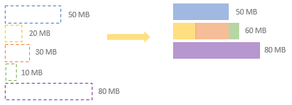
With the target size ready, the CoalesceShufflePartitions rule can start to coalesce the partitions according to the target size and to define the coalesced partition specs (CoalescedPartitionSpec) which will be used to create shuffle reader later. Let’s use an example to explain this process. As the diagram shows below, we have a shuffle operation with two input partitions on the map side. When the CoalesceShufflePartitions rule is not applied, the shuffle data are read into five output partitions, even though some of them are small.

When the CoalesceShufflePartitions rule is applied, it gets the size statistics of all shuffle partitions from the MapOutputStatistics collected at the map stage. In our example, we have two shuffles, each of which has five shuffle partitions:

The CoalesceShufflePartitions rule will make a pass through all the shuffle partitions, sum up the total size of a partition from all the shuffles, pack shuffle partitions with continuous indices to a single coalesced partition until adding one more partition would be over the target size. In our example, we use the default advisory target size (64MB) as the target size. The total size of the first shuffle partition is 50MB. The attempt to coalesce the first and the second shuffle partition (20MB) ends up a coalesced partition size (70MB) to be larger than the target size. Therefore, the two partitions cannot be coalesced and the first partition will be output as a separate output partition. A ColeascedPartitionSpec object is created for the first partition with the startReducerIndex as 0 (inclusive) and the endReducerIndex as 1 (exclusive).

The CoalesceShufflePartitions rule moves on to add the second and the third partitions, resulting at 50MB which is smaller than the target size.

The fourth partition is then added as well and the total size of second, third and fourth partition (60MB) is still not over the target size.

The attempt to add the fifth partition ends up a partition size (140MB) which is over the target size. Therefore, the second, thrid and fourth partitions are coalesced into one partition (60MB). A CoalescedPartitionSpec object is created which has the startReducerIndex as 1 and the endReducerIndex as 5.

As there is no further partition to process, another CoalescedPartitionSpec is created for the last (fifth) partition. Eventually, we have three output partitions now including the one made up with the three small partitions.
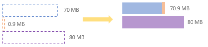
The example above shows the normal scenario where small partitions are coalesced as long as their total size is not over the target size. However, there is an exception scenario where a partition is smaller than the minPartitionSize but the partitions adjacent to it on both sides will exceed the target size if adding the small partition. For this scenario, the small partition will be merged with the smaller one between the two adjacent partitions.
At this point, the CoalesceShufflePartitions rule created a sequence of CoalescedPartitionSpec objects, each of which defines the spec for one of the output partition. These partition specs will be used by the shuffle reader to output partitions accordingly. The CoalesceShufflePartitoins rule creates an AQEShuffleReadExec operator which wraps the current shuffle query stage and creates the ShuffledRowRDD with the CoalescedPartitoinSpecs defined above. For each partition of the ShuffledRowRDD, which is defined by one CoalescedPartitionSpec, a shuffle reader is created to read shuffle blocks from the range of map output partitions defined by the startReducerIndex and endReducerIndex of the CoalescedPartitionSpec.
Internally, the getMapSizesByExecutorId method of MapOutputTracker is called to get the metadata of the shuffle blocks to read, including block manager id, shuffle block id, shuffle block size, and map index. A BlockStoreShuffleReader is then created, which initialises a ShuffleBlockFetcheriterator for conducting the physical read operations to fetch blocks from other nodes’ block stores.
Dynamically optimizing skew joins
With a good understanding of the previous section that explains the dynamic shuffle partition coalescence, it would be easy to understand the dynamic skew join optimisation, which is kinda the “reversed” operation of the partition coalescence that splits a skewed partition into multiple smaller partitions.
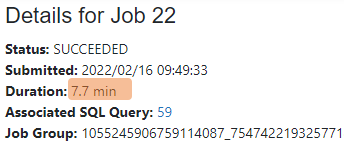
The example below shows a job execution with skewed partition. As you can see, the skewed partition has 5.8GB data while the other partitions only have less than 20MB data. It takes 6.7 minutes to run the task of the skewed partition while less than 1 second is used to run the tasks of the other partitions. The long running time of the task with skewed partition makes the total job execution time to be 7.7 minutes.

We then enable the AQE with the dynamic skew join optimisation applied and rerun the same query again. As the skewed partition has been split into multiple small partitions, the largest partition is now 234MB and it takes 29 seconds to run the partition. Thanks to the increased parallelism, the total job execution time is reduced from 7.7 minutes to 1 minute.


The OptimizeSkewedJoin rule is the AQE optimizer responsible for dynamic skew join optimisation. At a high level, this rule splits a skewed partition and replicate its matching partition on the other side of the join so that more tasks are created to do the join in parallel to avoid straggler tasks which slows down the job completion.

Internally, the OptimizeSkewedJoin rule first checks whether or not the join to optimise is either a sort merge join (SortMergeJoinExec) or a shuffle hash join (ShuffledHashJoinExec). Only these two types of join are supported by the OptimizeSkewdJoin rule in Spark 3.2.
Next, the OptimizeSkewedJoin rule detects the skewed partitions. A partition is considered as a skewed partition if it is larger than the specified skewed partition threshold (spark.sql.adaptive.skewJoin.skewedPartitionThresholdInBytes, default 256MB) and it is larger than the median partition size multiplying the skewed partition factor (spark.sql.adaptive.skewJoin.skewedPartitionFactor, default 5).

After the skewed partitions are found, we can then calculate the target size of the split partitions which is either the average size of non-skewed partition or the advisory partition size (spark.sql.adaptive.advisoryPartitionSizeInBytes, default 64MB) depends which one is larger.
The OptimizeSkewedJoin rule defines partition splits according to the map output sizes and the target size. It first gets the sizes of all the map outputs for the shuffle of the skewed partition. It then makes a pass through all the map output sizes, one by one, and makes attempts to merge the adjacent map output sizes so that the map outputs are grouped with their summed size close to the target size. A PartialReducerPartitionSpec is then created for each group, which encapsulates the id of reducer (for the skewed partition), the start map index (the start index of the map output in the group) and the end map index (the end index of the map output in the group).

Now the OptimizeSkewedJoin rule has the list of PartialReducerPartitionSpecs ready for creating the physical AQEshuffleReadExec operator. The remaining steps for physical shuffle blocks readings are mostly same as the steps mentioned earlier for coalescing shuffle partitions. The main difference is that the shuffle reader created by the OptimizeSkewedJoin rule specifies the startMapIndex and the endMapIndex for the list of map outputs to read.
While the skewed partition is split into multiple smaller partitions, its matching partition on the other side of the join are replicated to the same number of copies matching the number of the split partitions. The join happens between one split of the skewed partition and one copy of the replicated partition.
