
One of the reasons — actually, the core reason — I chose DolphinDB as the built-in streaming engine for QuantFlow’s streaming execution layer is that it’s really fast, even for the kind of complicated computation that requires chained steps. Thanks to that speed, and with QuantFlow’s MarketState engine and FeatureDAG compiler on top, we can leverage Grafana’s visualization capability to set up a real-time market monitor dashboard with almost no effort.
What QuantFlow Actually Does
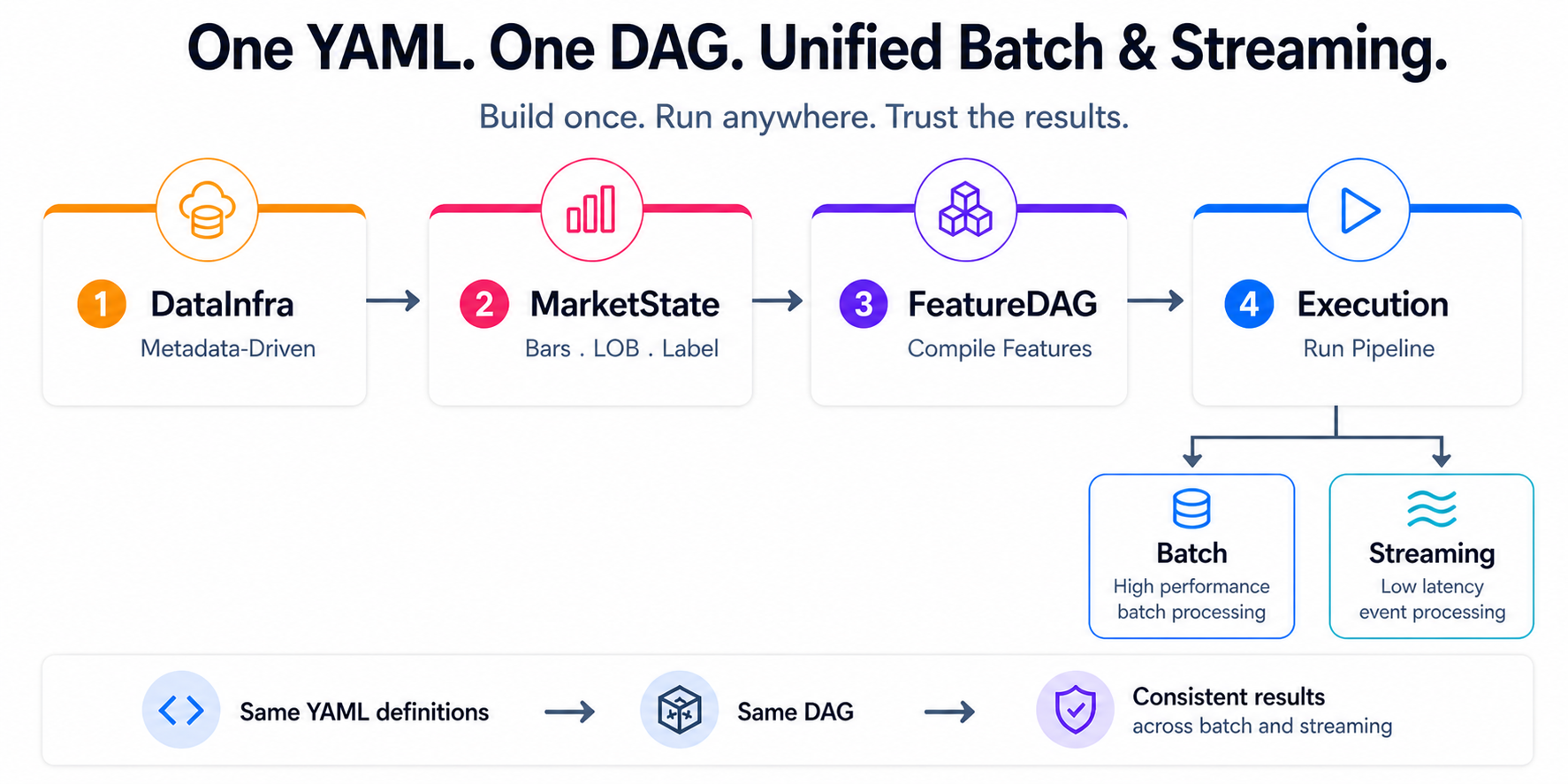
The drive behind QuantFlow is simple: help quant teams set up their research and trading foundation in days instead of months. The idea is to transform raw market data into research- and production-ready machine learning features, with the same pipeline running consistently across batch (research) and streaming (trading) from a single set of YAML definitions.
It’s a unified declarative pipeline. Ingestion → CDM normalization → market state reconstruction → feature compilation → execution. Define it once. Run it anywhere.
How the Streaming Path Works
QuantFlow parses user requirements — defined in YAML — and generates a corresponding IR DAG that represents the full feature computation graph: rolling windows, lags, arithmetic, conditional logic, array extractions from order book data, all expressed as a directed acyclic graph of operations. The batch path compiles this DAG into Polars expressions. The streaming path compiles the exact same DAG into DolphinDB reactive engine scripts.
This is where DolphinDB shines. Each computation step becomes a metric expression inside a ReactiveStateEngine. Multiple features sharing the same input table get consolidated into a single engine — the FeatureDAG compiler inlines intermediate expressions and merges compatible features together. So instead of deploying one engine per feature, we deploy a handful of consolidated engines, each producing multiple output columns in one pass.
The engines communicate through shared stream tables. An upstream engine writes rows; a downstream engine subscribes and reacts. Everything stays in memory, inside the same DolphinDB process. No serialization between steps. No disk. No context switches. The pipeline deploys, Python steps aside, and the whole thing runs server-side.
Setting Up the Dashboard
DolphinDB ships a Grafana datasource plugin that talks WebSocket directly to the server. This means your dashboard queries execute inside the same DolphinDB process that’s computing the features — no REST API, no middleware, no serialization.
Setup takes three steps.
1. Pull the DolphinDB Grafana image:
docker pull dolphindb/dolphindb-grafana:9.1.0docker run -d --name ddb_gra -p 5000:3000 dolphindb/dolphindb-grafana:9.1.0
This bundles Grafana 9.1.0 with the DolphinDB plugin pre-installed.
2. Add the data source. Log in at http://localhost:5000 (admin / admin), go to Configuration → Data Sources → Add, search “dolphindb”. The URL uses WebSocket format:
ws://host.docker.internal:8848
(Use host.docker.internal if DolphinDB runs on the host; use the container name if it’s in Docker too.)
3. Build the Dashboard. Create panels on a Grafana dashboard, write DolphinDB queries to query the stream tables generated by QuantFlow, and work on the visualization.
4. Finally, start the QuantFlow streaming pipeline.
