
From this blog post, I am starting to write about streaming processing, focusing on Spark Structured Streaming, Kafka, Flink and Kappa architecture. This is the first blog post of the Spark Structured Streaming deep dive series. This blog post digs into the underlying, end-to-end execution flow of Spark streaming queries.
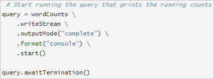
Firstly, let’s have a look at the official structured streaming query example from Spark:


A typical streaming query is defined in three steps: firstly create a data stream reader in the current Spark session that will be used to read streaming data in as a Spark DataFrame, then define the transforms on the DataFrame based on the processing requirements, and finally define the data stream writer and start running the query.
Now, let’s look into how a streaming query is executed by the Spark Structured Streaming framework under the hood.

SparkSession provides a ‘readStream‘ method which can be used by end-user developers to create and access an DataStreamReader instance that is responsible for loading an input stream from external data source. The data source format and input schema can be specified in the data stream reader. The ‘load‘ method of the data stream reader defines the Spark DataFrame which logically representing the input stream.
The transformation of the DataFrame that represents the data processing logics can be defined by the end-user developers by calling the operations available on the DataFrame. Most of the common operations available for batch processing are also supported for stream processing. Here is a list of unsupported operations. Just as how it works in the batch processing workloads, the DataFrame operations for streaming processing are also executed in the lazy mode. Under the hood, a Dataframe represents a logical plan which defines the computations required for the data processing. The computations will only be triggered when an action is invoked.
After data transformations of the DataFrame are defined, a DataStreamWriter instance needs to be created for saving the processed streaming data out into external storage. The DataStreamWriter can be created by calling the ‘writeStream‘ method of the DataFrame. The end-user developers can specify the output mode for writing the data into streaming sink, the partitions of the sink file system where the data written into, and the trigger for the micro-batch streaming jobs. Up to this point, all we have done is just to define the streaming query execution. The physical streaming query execution starts when the ‘start’ method of the DataStreamWriter is called.
The ‘start‘ method of the DataStreamWriter first creates the sink instance which supports continual writing data into external storage, and then passes the sink instance to the StreamingQueryManager of the current Spark session to create and start a StreamExecution instance. The StreamExecution instance is the core component that manages the lifecycle of a streaming query execution. There are two concrete implementations of the StreamExecution (which itself is defined as an abstract class), including the MicroBatchExecution and the ContinuousExecution. The micro-batch processing mode, i.e., processing data streams as a series of small batch jobs, implemented by MicroBatchExecution is the primary stream processing mode supported by Spark Structured Streaming engine. This mode supports exactly-once fault-tolerance guarantees and is capable to achieve end-to-end latencies at 100ms level. The ContinuousExecution supports the low-latency, continuous processing mode that achieves end-to-end latencies at 1ms level. However, this mode only supports map-like operations and can only achieve at-least-once guarantees. This blog post focuses on the micro-batch processing mode. I will dedicate a few blog posts to continuous processing mode in future.
Now, let’s look into a bit deeper on how StreamQueryManager creates and runs a streaming query (i.e. a StreamExecution instance). StreamingQueryManager is responsible to manage all the active streaming queries in a Spark session. It comes with an ‘activeQueries‘ hash map which caches the reference to the active streaming queries. The ‘start’ call from the DataStreamWriter will trigger the ‘startQuery‘ method which conducts three major activities in order, including defining streaming query (i.e. creating the StreamExecution instance), registering the created StreamExecution instance in the activeQueries hash map, and invoking the ‘start’ call of the StreamExecution instance.

To create a streaming query, logical plan of the DataFrame which is defined earlier with the required transformation operations is analysed. Please refer to my earlier blog post for more details of the Spark Catalyst Analyzer. With the analysed logical plan along with other streaming writing configurations, such as sink, output mode, checkpoint location and trigger), a WriteToStreamStatement is created which is the logical node representing a stream writing plan. After the WriteToStreamStatement is analysed, depending on the trigger type (ContinuousTrigger or not), one of the StreamExecution implementation classes, ContinuousExecution or MicroBatchExecution, is created to manage the stream query execution. The created streaming query is then registered in the activeQueries.
After that, the ‘start’ method of the created StreamExecution instance is called to start a separate thread to run the streaming querying which executes repeatedly each time when new data arrives at any source specified in the query plan. Within the thread, after the initialisation of source and metadata objects, the ‘runActivatedStream‘ method is called. The execution flow of the ‘runActivatedStream‘ method is defined in each implementation class of the StreamExecution. The rest of the blog post looks into the implementation of this method of the MicroBatchExecution. However, before digging into the method, let’s have a step back and have a look at the core components in the Sparking Structured Streaming system.

Firstly, we have external streaming sources and sinks which support continuous data read and write. Within the Spark Structured Streaming framework, there are three main components: the Source interface which abstracts the data read from the external streaming sources, the Sink interface which abstracts the data write into the external Streaming sinks, and the StreamExecution which manages the lifecycle of streaming query executions. The Source interface defines three core methods for communicating with external data sources, getOffset(), getBatch(), and commit(), while the Sink interface defines one core method for output the streaming data to sink, addBatch(). I will discuss those methods in details in the subsequent blog posts which digs into the sources and sinks implementation in the Spark Structured Streaming framework.
The execution flow of each micro-batch data processing is defined in the ‘runActivatedStream‘ method of the MicroBatchExecution class. A TriggerExecutor (ProcessingTimeExecutor by default) instance, is created to schedule and trigger micro-batch processing jobs. I draw the following diagram to depict the end-to-end execution flow of a micro-batch job.

(1) The execution of micro-batch processing starts from identifying the start offsets to read from the sources. The start offsets are determined based on the last batch execution recorded in the OffsetLog and CommitLog. The OffsetLog is a Write-Ahead Log (WAL) recording the offsets of the current batch before the batch run while the CommitLog records the batch commit when the batch run is completed successfully. If the last batch id recorded in the OffsetLog equals to the last batch id recorded in the CommitLog, it implies the last batch was successfully processed, so the start offsets of current batch == the end offsets of the last batch. If the last batch id recorded in the OffsetLog equals to the last batch id recorded in the CommitLog + 1, it implies the last batch was failed and needed to rerun, so the start offsets of current batch == the start offsets of the last batch.
(2) Check each source whether new data is available and get the next available offset.
(3) Construct next batch, record the range of offsets that the next batch will process in the WAL OffsetLog.
(4) Call the getBatch method of the sources to return the DataFrame that represents the data between the start offsets and end offsets. Note that no physical data is actually read from the source at this moment, but instead the getBatch method only returns the data plan of the batch.
(5) Replace sources in the logical plan of this stream query with the data plan of the new batch to get the newBatchesPlan. Rewire the newBatchesPlan to use the new attributes that were returned by the sources to get the newAttributePlan.
(6) Create triggerLogicalPlan from newAttributePlan. Convert the newAttributePlan to WriteToMicroBatchDataSource if required.
(7) Create the IncrementalExecution for the current batch run with the triggerLogicalPlan as input. IncrementalExecution is a variant of the QueryExecution (please refer to my earlier blog post) for planning stream queries that allow incremental execution of a given logical plan. Just like the batch query planning, the stream query planning also needs to go through the same planning stages which will be covered in details in the subsequent blog posts in this series.
(8) Based on the generated execution plan, a new Dataset that logically represents the next batch is created.
(9) Add the next batch Dataset to the sink through addBatch method provided by the Sink interface.
(10) Log the batch execution into the CommitLog to record this successful batch run.
