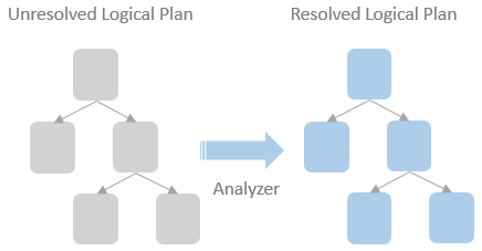
After the SparkSQLParser parses a SQL query text into an ANTLR tree and then into a logical plan, the logical plan at this moment is unresolved. The table names and column names are just unidentified text. Spark SQL engine does not know how those table names or column names map to the underlying database objects. Catalyst provides a logical plan analyzer, which looks up SessionCatalog and translates UnresolvedAttributes and UnresolvedRelation into fully typed objects.

Apart from the relations and attributes resolution, Catalyst Analyzer is also responsible for validating the syntactical correctness of the Spark query and conducting syntax-level operators and expressions analysis. As mentioned in the last blog post, a LogicalPlan is internally represented as a tree type in Catalyst. A set of analysis rules has been defined by the Catalyst Analyzer, which will be pattern matched with the node in the LogicalPlan tree and applied the analysis rules to the matched node.
In Spark 3.0.0, Catalyst Analyzer ships with 51 built-in rules, which is organised into 12 batches. In the rest of this blog post, I will focus on the two of the most important rules, ResolveRelations and ResolveReferences, but also choose some other representative rules to introduce.

ResolveRelations
ResolveRelations rule replaces UnresolvedRelations with relations from the catalogue. Taking the following Spark SQL query as an example, two tables are involved in the query, [sales] and [items]. SparkSQLParser parsed those two tables as two UnresolvedRelations.
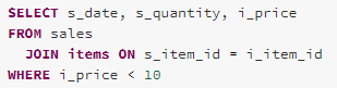

What the ResolvedRelation rule needs to do is to translate the UnresolvedRelations to Relations with full type information. As you can see from the snapshot below, the full qualified data table name and the tables’ column names need to be resolved from the table metadata stored in the SessionCatalog.

When the ResovledRelation rule is being applied to our query (LogicalPlan), the resolveOperatorsUp method of the logical plan is called, which traverses through all the nodes bottom-up and call the lookupRelation method for UnresolvedRelations node.
The lookupRelation method looks up the concrete relation of the UnresolvedRelation from the session catalog. The loadTable method from CatalogV2Util loads table metadata by the identifier of the UnresolvedRelation and returns a Table type, which represents a logical structured data set of a data sourice, such as a directory on the file system, a topic of Kafka, or a table in the catalog.

If a V1 table is found in the catalog, the getRelation method of the v1 version session catalog (from catalogManager.v1SessionCatalog) is called, which creates a View operator over the relation and wraps it in a SubqueryAlias that tracks the name of the view. If a V2 table is found in the catalog, a DataSourceV2Relation object is created, which will also be wrapped by a SubqueryAlias that tracks the relation name. SubqueryAlias is a unary logical operator, which hosts an alias of the subquery it wraps that can be referenced by the rest of the query.

ResolveReferences
ResolveReferences rule replaces UnresolvedAttributes with concrete AttributeReferences from a logical plan node’s childern. When ResolveReferences rule is applied to a logical plan, the resolveOperatorsUp function traverses and applies the rule to the nodes of the logical plan from the bottom up. The rule will only be applied if all of a node’s children have been resolved. Therefore, you can see that a logical plan with multiple levels of children cannot be solved in a single run of the rule, but instead, multiple runs are required until the logical node tree reaches the fixed point.

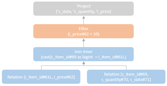
In our SQL query example mentioned above, the ResolveRelations rule has resolved the UnresolvedRelation ‘sales’ and ‘items’ to resolved relation with resolved attribute references to the underlying data source columns. When the ResolveReferences rule is applied, only the “Join” node’s children are solved, so only the unresolved attribute references with the “Join” node are solved. The “Filter” node is not qualified to solve in this current iteration run.

In the next iteration run, the “Join” node has been marked as resolved, and the requirement for applying the ResolveReferences rule on the “Filter” node is met. The ‘i_prece’ attribute can now be resolved.
Internally, the mapExpression method of the current logical plan to resolve is called to run resolveExpressionTopDown function on all the expressions of the logical plan. If any expression is UnresolvedAttribute type, the name parts of the unresolved attributes will be resolved to a NamedExpression using the input from all child nodes of this logical plan.

Some More Examples
CTESubstitution
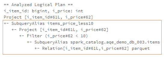
CTESubstitution rule is used to analyse the WITH SQL syntax that substitutes a WITH node as subqueries. The apply method of CTESubstitution rule calls the traverseAndSubstituteCTE method, which substitutes CTE definitions from last to first as a CTE definition can reference a previous one.
From the example below, we can see the UnresolvedRelation, which references a CTE definition, is replaced by the logical plan of the CTE definition.


ResolveJoinStrategyHints
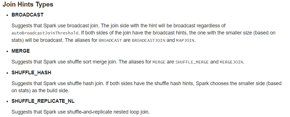
ResolveJoinStrategyHints rule analyses the join strategy hint on a relation alias by recursively traversing down the query plan to a relation or subquery that matches the specified relation alias and wraps it using ResolvedHint node. Here is a list of supported join hints types from Spark official doc.
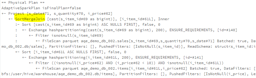
Takes our ‘sales’ and ‘items’ table join SQL query mentioned above as an example, the SortMergeJoin is chosen for the join.
We now add the BROADCAST join hint on “items” relation.

In the analyzed logical plan, a ResolvedHint node with strategy as broadcast is added and wraps with the “items” relation node.

If we check the physical plan, we can see the join type has been changed from sort merge to broadcast.

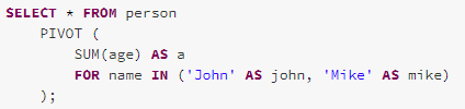
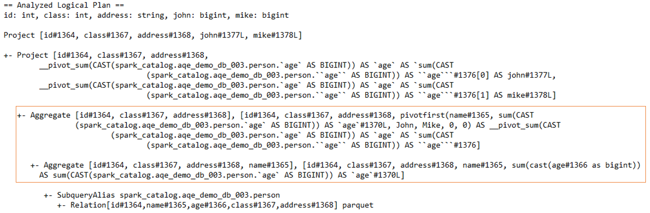
ResolvePivot
ResolvePivot rule converts a PIVOT operator into a two-stage aggregation. the stage aggregates the dataset using agg functions grouped by the group-by expression attributes (Group-by expressions coming from SQL are implicit and need to be deduced) and the pivot column. The pivot column will only have unique values after the first stage. The PivotFrist function is then used to rearrange to pivot column values into the pivoted form. The second aggregate is then called to aggregate the values by the pivoted agg columns.
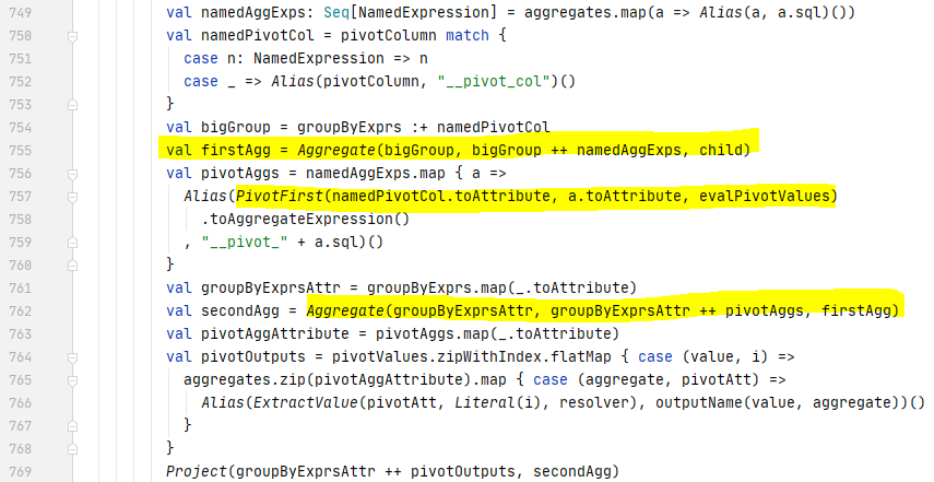
Take the following query as an example, the Pivot operator is converted into two Aggregate operators, the first one Aggregate makes the pivot column ‘name’ containing unique values, and the second one converts the pivot values (‘John’ and ‘Mike’) to the columns and aggregates (sum) on the ‘age’ column.