In this blog post, I am going to explain the Join strategies applied by the Spark Planner for generating physical Join plans.

Based on the Join strategy selection logic implemented in the JoinSelection object (core object for planning physical join operations), I draw the following decision tree chart.

Spark SQL ships five built-in Join physical operators, including:

• BroadcastHashJoinExec
• ShuffledHashJoinExec
• SortMergeJoinExec
• CartesianProductExec
• BroadcastNestedLoopJoinExec

The Join strategy selection takes three factors into account, including:

• Join type is equi-join or not
• Join strategy hint
• Size of Join relations

This blog post first explains the three factors and then describes the join strategy selection logic based on the considerations of those three factors, including the characteristics and working mechanism of each join operator.

Selection Factors

Equi-Join or Not

An Equi-Join is a join containing only the “equals” comparison in the Join condition while a Non Equi-Join contains any comparison other than “equals”, such as <, >, >=, <=. As the Non Equi-Join needs to make comparisons to a range of unspecific values, the nested loop is required. Therefore, Spark SQL only supports Broadcast nested loop join (BroadcastNestedLoopJoinExec) and Cartesian product join (CartesianProductExec) for Non Equi-Join. Equi-Join is supported by all five join operators.

Spark SQL defines the ExtractEquiJoinKeys pattern, which the JoinSelection object uses to check whether a logical join plan is equi-join or not. If it is equi-join, the elements of the join are extracted from the logical plan, including, join type, left keys, right keys, join condition, left join relation, right join relation and join hint. The information of those elements forms the basis for the following join planning process.

Join Hints

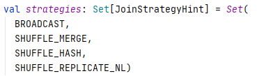
Spark SQL providers end-user developers some controls over the join strategy selection through Join Hints. For Spark 3.0.0, four join hints are supported, including:

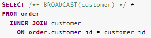
The end-user developers can add the Hint syntax with the hint type and target table in the SELECT clause.

An UnresolvedHint node is generated by the parser and converted into a ResolvedHint node by the Analyzer.

The Optimizer applies the EliminateResolvedHint rule which moves the hint information into the join operator and removes the ResolvedHint operator.

The join hint information is extracted by the ExtractEquiJoinKeys pattern mentioned above and used in the join strategy selection process which will be explained later in this blog post.

Size of Join Relations

The last but not least factor for selection join strategy is the size of the join relations. The core principle for join strategy selection is to avoid reshuffle and reorder operations which are expensive and affect the query performance badly. Therefore, the join strategy without the need for reshuffle and/or reorder, such as the hash-based join strategies, is preferred. However, the usability of those join strategies depends on the size of the relations involved in the join.

Now that we have known the factors we need to take into account when selecting a join strategy, the rest of this blog post will look into the selection logic and the join operators.

Equi-Join

Compared to the Non Equi-join, Equi-join is much more popular and commonly used. All the five join operators mentioned earlier support Equi-join. The portion of the decision tree chart below depicts the logic used for selecting join strategy for Equi-join. The candidate join strategies are searched in the order of possible join performance. The first strategy that meets the selection condition is returned and the search is terminated and will not consider the other strategies.

Select by Join Hint

The join hint specified by the end-user developers has the highest priority for join strategy selection. When a valid join hint is specified, the join strategy is selected based on the following condition:

• For BROADCAST hint, select the BroadcastHashJoinExec operator. when BROADCAST hint is specified on both sides of the join, select the smaller side.
• For SUFFLE_HASH hint, select the ShuffledHashJoinExec operator. when SUFFLE_HASH hint is specified on both sides of the join, select the smaller side.
• For SUFFLE_MERGE hint, select the SortMergeJoinExec operator if the join keys are sortable.
• For SUFFLE_REPLICATE_NL, select the CartesianProductExec operator if join type is inner like.

If no join hint is specified or the join condition is not met for the specified join hint, the selection flow moves down the decision tree.

Broadcast Hash Join

Broadcast hash join (with the BroadcastHashJoinExec operator) is the preferred strategy when at least one side of the relations is small enough to collect to the driver and then broadcast to each executor. The idea behind the Broadcast hash join is that the costs for collecting data for a small relation and broadcasting to each executor are lower than the costs required for reshuffle and/or reordering. For Broadcast hash join to have good performance, the relation to broadcast has to be small enough, otherwise, the performance can get worse or even end up with Out-Of-Memory errors. The default size threshold for a relation to use Broadcast is 10MB, i.e. the relation needs to be smaller than 10MB. The default size can be adjusted by configuring the spark.sql.autoBroadcastJoinThreshold setting based on the available memory in your driver and executors.

Internally, the BroadcastHashJoinExec overrides the requiredChildDistribution method and declares the broadcast distribution requirement of the relation to broadcast.

When the EnsureRequirements rule is being applied before the actual execution, a BroadcastExchange physical operator is added before the execution of join.

When the BroadcastExchange operator is being executed, it first collects the partitions of the relation for broadcasting to the Driver.

If the total row number of the relation is smaller than the MAX_BROADCAST_TABLE_ROWS threshold, the relation will be broadcasted. The MAX_BROADCAST_TABLE_ROWS threshold is set to 341 million rows, which is 70% of the BytesToBytesMap maximum capability. Note that this threshold is different from the spark.sql.autoBroadcastJoinThreshold (10MB by default). The MAX_BROADCAST_TABLE_ROWS threshold is used to control the broadcast operation during the broadcast exchange, while the spark.sql.autoBroadcastJoinThreshold is to control the selection of Broadcast Hash Join strategy.

If the row number of the relation is smaller than the MAX_BROADCAST_TABLE_ROWS threshold, a copy of the relation data is sent to each executor in the form of a broadcast variable of HashedRelation type.

On the executor side, the broadcasted relation is used as the BuildTable of the join, and the relation originally exists in the executor, which is the larger table of the join, is used as the StreamTable of the join. The join process iterates through the StreamTable, and look up the matching row in the BuildTable.

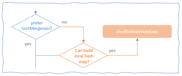
Shuffle Hash Join

If the condition for selecting Broadcast Hash Join strategy is not met, the selection flow moves to check whether the Shuffle Sort Merge strategy is configured as preferred or not. if not, it exams whether the condition for using Shuffle Hash Join strategy is met.

To be qualified for the Shuffle Hash Join, at least one of the join relations needs to be small enough for building a hash table, whose size should be smaller than the product of the broadcast threshold (spark.sql.autoBroadcastJoinThreshold) and the number of shuffle partitions.

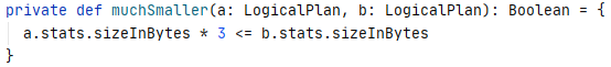
In addition, the small relation needs to be at least 3 times smaller than the large relation. Otherwise, a sort-based join algorithm might be more economical.

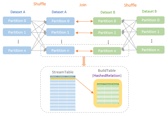
The shuffle Hash Join strategy requires both relations of the join to be shuffled so that the rows with the same join keys from both side relations are placed in the same executor. A hashedRelation is created for the smaller relation and is used as the BuildTable of the join. The larger relation is used as the StreamTable.

Shuffle Sort Merge Join

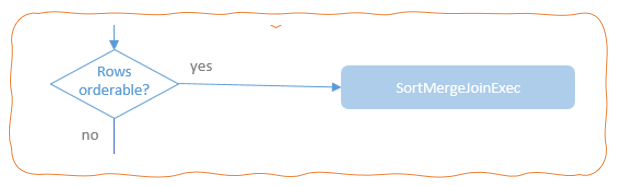
If the condition for selecting Shuffle Hash Join strategy is not met or the Shuffle Sort Merge strategy is configured as preferred, the selection flow moves on to exam whether the condition for using Shuffle Sort Merge strategy is met. To use the sort-based join algorithm, the join keys have to be orderable.

Unlike the hash-based sorting algorithms which require loading the whole one side of join relations into memory, the Shuffle Sort Merge Join strategy does not need any join relations to fit into the memory, so there is no size limit for the join relations. Although the sort-based join algorithm is normally not as fast as the hash-based join, it normally performs better than the nested loop join algorithms. Therefore, the Shuffle Sort Merge Join takes the middle position for both the performance and flexibility considerations.

The Shuffle Sort Merge Join strategy also requires both relations of the join to be shuffled so that the rows with the same join keys from both side relations are placed in the same executor. In addition, each partition needs to be sorted by the join key in the same ascending order.

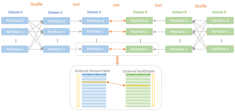
Either of the two join relations can be used as StreamTable or BuildTable. When a relation is used as the StreamTable of the join, it is iterated row by row in order. For each StreamTable row, the BuildTable is searched row by row in order as well to find the row with the same join key as the StreamTable row. As both the StreamTable and BuildTable are sorted by the join keys, when the join process moves to the next StreamTable row, the search of the BuildTable does not have to restart from the first BuildTable row, but instead, it just needs to continue from the BuildTable row matched with the last StreamTable row.

Cartesian Product Join

If the condition for selecting Shuffle Sort Merge strategy is not met and the JoinType of the join is InnerLike, Cartesian Product Join is selected. This normally happens for a Join query with no join condition defined. At the core, the Cartesian Product Join is to calculate the product of the two join relations. As you can imagine, the performance of Cartesian Product Join could get really bad for large relations, so this type of join should be avoided.

Broadcast Nested Loop Join

When the conditions for selecting all of the other four join strategies are not met, the Broadcast Nested Loop Join strategy is selected. The join process of this strategy involves a nested loop of the StreamTable and the BuildTable.

The performance of this strategy can get really bad. An optimisation made to this strategy is to broadcast the relation when it is small enough for broadcasting.

Non Equi-Join

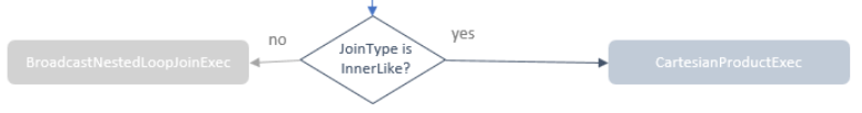
If the join to plan is not an Equi-Join, the selection flow works as the following portion of the decision tree shows.

There are only two Join strategies supporting Non Equi-Join type, the Cartesian Product Join and the Broadcast Nested Loop Join.

If a Join Hint is specified in the join query, select the corresponding Join strategy according to the Join Hint. Otherwise, if one or both sides of relations are small enough to broadcast, select the Broadcast Nested Loop Join strategy and broadcast the smaller relation. If no relation is small enough to broadcast, check whether the JointType is InnerLike or not. If so, select the Cartesian Product Join strategy. Otherwise, fall back to the There are only two Join strategies supporting Non Equi-Join type, the Cartesian Product Join and the Broadcast Nested Loop Join strategy as the final solution.

• *Deep Dive - Spark SQL Query Engine
• Databricks / Spark