• Buy-Side Financial Data Models (1) – Overview
• Buy-Side Financial Data Models (2) – Financial Instruments

This is the first blog post of the “Buy-Side Financial Data Models” series I am planning to write. To kick off this blog series, this post provides a high-level overview of the core data domains, unified data modelling, and layered data model implementation for buy-side asset management business. In the following posts of this blog series, I am going to dive into the data details of those data domains.

Core Data Domains

The term “Data Domain” has been overused to refer to some different things. To avoid confusions, the “Data Domain” used here refers to a logical group of data that share a conceptually common meaning or purpose. The use of Data Domain helps data professionals and business users to build a global view on the data they can utilise.

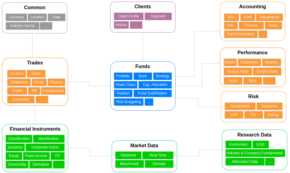
For the buy-side asset management business, I summarise the following ten data domains.

“Funds” domain is the core data domain that contains data for representing main entities, configurations, administrations involved in the fund management lifecycle. The first type of data in this domain is the data entities that represent the core components involved in the business processes, such as Funds, Portfolios, Books, Strategies, Positions, and Accounts. Those data entities sit at center and are commonly shared and referenced across the entire organisation for the major business activities, such as trading, accounting, performance analysis, and risk management. Funds domain also contains data for fund configurations (such as Share Classes, Capital Allocations, and Risk Budgeting) and fund administration processes (such as client fund subscriptions, redemption etc).

The data in the funds domain are normally defined/edited in the main IMS (Investment Management System) or PMS (Portfolio Management System), such as Charles River and Murex, the backbone operational systems for an asset management business. Periodical ETL jobs or event-driven streaming jobs export/sync the data from the operational data store to an analytical data store. Those data are normally well structured with fixed and clearly defined schema that makes the relational databases with tabular model the optimal way to host them.

As those core data entities in this domain are common and shared across the major business processes, they are the natural candidates for the conformed dimension role that can be used to dice and slice measures/metrics for the different business activities operating in this organisation. For many of those data entities, the historical versions of the records in those data entities need to be persisted. Those data entities therefore need to be modelled as type 2 slowly changing dimensions (SCD) that add a new row for any new value and maintain the existing row unchanged while the row is being updated.

“Financial Instruments” domain is another core data domain in asset management business. Similar to the the “Goods” traded in a supermarket, financial instruments are the “Goods” traded by asset managers in a financial market. Just like the classification and specification details of those goods are essential for a supermarket’s daily operations and all sorts of business processes, financial instrument classification and specification details are the core reference data used across asset management business processes, such as researching, trading, portfolio managing, accounting, performance attributing, risk managing, etc.

The financial instrument reference data is normally governed with a Sec Master tool, such as GoldenSource, which integrates instruments reference data of all sorts of asset classes from different data vendors, such as Bloomberg, ICE, CBOE, Refinitive, FactSet, etc, and masters and stores the data in an operational data store, and publishes the single-truth, golden-copy data across the organisation, to ensure all the functions, from front-office to mid/back-office, are using consistent data.

One main challenge to manage financial instrument reference data is caused by the heterogeneousness between different asset classes. The instruments between different asset classes often have very different attributes, such as between a stock share and a bond. Even within the same asset class, the attributes of different financial instruments might be very different, such as ABS and CDO. This raises the challenge to design an effective, maintainable and flexible data model to organise and serve the financial instrument reference data. After the extensive efforts on analysing FIBO (Financial Industry Business Ontology), CFA official books, and other standards, I put together the following classifications in the diagram below. I plan to write about the financial instrument data domain from the next blog post, to discuss the modelling and also dive into the core instrument attributes of each asset class.

“Market Data” domain contains the temporal price/quote/rate data of the financial instruments, which are the data directly related to the money-making, profit-generating frontier of investing businesses. The market data can represent the past (historical data) and now (real-time data) of the market consensus that support investors to predict the future (or make near to immediate future investing decision).

Similar to the financial reference data, the market data is also heterogeneous across different instruments due to the various dimensions required to represent different instruments. For example, while a normal stock market price data is identified by time and issuer, an option contract price data needs to be identified by additional dimensions, like strike price, expiration date, call/put etc. Unlike the financial instrument reference data, the volume of market data is big and data query performance requirement is high.

There are a number of ways to model and store the market data. For historical data with data snap frequency > 1 hour:

• create a dedicated table per instrument type with schema specifically defined to fit the dimensions of the instrument type. The old systems normally use a relational database to host those tables. To ensure a satisfied query performance with the large data volume, those tables need to be partitioned (normally by the snap date) and indexed (normally by the dimensions). Nowadays, those tables can be created in the big data supported, Lakehouse type data platform, such as Snowflake and Databricks. Considering the number of instrument types, a significant efforts are required to create and maintain those tables.
• a unified key-value type table for all instrument types. Apart from the fields for identifying a specified instrument and the snap time, each row contains a key field for the name of the dimension (or name of the quote/rate) and a value field for the value of the dimension (or value of the quote/rate). A full piece of market data for a instrument consists of multiple rows which can be pivoted into a single record row to serve the queries from consumers. With properly designed partitioning and indexing, for instruments that don’t require high snap frequency, such as fixed income and derivatives, a relatively satisfied query performance can be achieved. The advantage of this design is the less efforts required for maintain a separate table for each instrument type.
• store the market data in a semi-structured data format, such as JSON. A document database, such as MongoDB, can be used to host those data. Another option is to store those data in a Lakehouse that supports JSON data type, such as the VARIANT type in Snowflake.

For high-frequency/tick-level market data which is required for backtesting or time series analysis, a time-series database is optimal. Apart from the fast but expensive KX kdb+, more and more alternatives are available, such as OneTick, DolphinDB, and InfluxDB.

“Research Data” domain contains the data required by all sorts of analysis for reaching investing decisions, such as economic indicators for macroeconomic analysis, market research data for industry analysis, and financial reports for company fundamental analysis.

Alternative data is another type of the research data that is attracting more and more attentions. Alternative data refers to the data from non-traditional sources, such as news, social media and IoT sensors. As it has became not that hard to access the traditional data sources, the market participants have relatively equal access to the information from traditional data sources and the market becomes more and more efficient. Alternative data provide opportunities for investors who are willing to spend efforts on exploring the alternative date to discovery additional information that might generate additional alpha.

Compared to the other data domains, a large portion of the data types in research data domain is unstructured or semi-structured. In addition, not only the volume of those type of data is often big, but also they contains a large and a variety number of attributes. The schema-on-write mode for traditional relational databases is not suitable to ingest and store those data. Instead, the schema-on-read mode that ingests and stores the data in their original format and extract schema as required when reading the data for consuming is more suitable.

In addition, with the advance of the AI technology and computing power over large datasets, new approaches to analyse research data, especially for those new types of alternative data are being applied, from the traditional “know question, seek answer” to the “don’t know question, but tell me”.

“Trades” data domain contains the data generated from the trading activities. The core data entity in this domain is the ‘Order’ data that is normally sourced from an Order Management System (or the Trading & Execution module of an integrated IMS). An order record holds the necessary information of a financial instrument buy or sell (or contract) attempt, such as security identifier, order type, price, quantity. Apart from those basic attributes of an order, an order record also holds the information of the status of the order processing, participants during the process and the timestamps. Those data are normally necessary for evaluating internal and external operation performance, such as evaluating external brokers’ performance on order executions and confirmations.

When order data extracted into the analytical data store from OMS, they are often denormalised into a wide table that containing all the information related to the order in one row. In addition, for each order status of a order record, a separate row is added so that the order details of each status can be kept. When an order is filled, the order is qualified to be a ‘”trade”. A separate ‘trade’ table is normally created in the analytical data store to hold the trades, even though most of the fields will be same with the corresponding order, that logically makes sense for the downstreaming consumers. In addition, an order might be filled by multiple trades due to liquidity and costs reasons, while multiple orders might be bundled and traded in one go. Therefore, that can be a many-to-many relationship between order table and trade table. When an order is filled, the “position” table (and other derived aggregate tables for accounting, performance, and risk) needs also update accordingly (don’t have to be immediately, but can happen during daily or hourly processing) .

The order and trade are the core transactional data that retains the trading information at the highest granularity level. They are the base for the higher-level, lower granular measures that can be derived according to specified business requirements for accounting, performance/risk evaluating, operation, compliance, management reporting etc. For sell-side business, there is a higher requirement to properly retain and manage those transaction data for all sorts of compliance reporting requirements: Best Execution, MiFIR transaction reporting, MAR/AML reporting, and also as data feeds for surveillance system, such as SteelEye, to detect potential market abusing activities. Furthermore, trade data carries rich information over the investors’ trading patterns/behaviours. Especially for a business serving retail investors, mining those information from trade data might lead to enormous profiting opportunities.

I also included the parties involving in the trade transaction process, such as PB, counterparty, custodian etc, in the trade domain, that can be modelled as dimensions to dice and slice the trade measures to their’s angles. Those data can also be put into a separate “Parties” domain, however, I consider that makes more sense to place the parties close to the process they are participating.

“Accounting” data domain includes the accounting data that contains the information representing the financial status of a fund and related financial transactions. This domain contains some core financial performance metrics, such as NAV, PnL, and AUM, that are calculated and reconciled (in-house or by external back-office service suppliers) periodically, daily, weekly, or monthly, depending on the reporting requirement and the complexities on valuating the current market values of the investment positions held by the fund, including those illiquid securities and OTC contracts that lack of market price information. After those metrics are calculated and loaded into the analytical data store, they will be enriched with additional attributes, such as those core data entities in the fund data domain mentioned above, so that those metrics (that are additive) can be aggregated, and diced and sliced by those attributes. NAV is calculated at Fund level which is not additive.

The accounting data domain also retains the transaction-level financial data, such as internal and external payments, account adjustment entries, etc. Those data can be directly extracted from the operational source systems where they are held and loaded into the analytical data store for the further aggregations and enrichment based on business requirements.

“Performance” data domain contains data for evaluating and reporting the investment performance of a fund at the different levels. Unlike the accounting data domain mentioned above that contains the data for evaluating financial performance of a fund, the data included in this domain mainly describes the risk and return characteristics of the investments. One thing to note is that the risk characteristics discussed here carry different meaning and serving different purpose compared to the risk metrics included in the “Risk” data domain we will talk about later. The risk characteristics discussed here is an integral part to evaluate and represent the performance of an asset investment, while the data in the “Risk” domain are the risk metrics representing the market, liquidity, counterparty, and other risks that might lead to fund losses.

There are a variety of return measures that are calculated with different formula and represent the return from different angles, such as holding period return vs annualised return, arithmetic return vs geometric return, time-weighted return vs money-weighted return (e.g., YTM for bond investment), gross return vs net return vs real return vs leveraged return, pre-tax return vs after-tax return. The risk of an asset can be evaluated by the volatility of returns from the asset with standard deviation as the common measure. The risk and return measures are not additive. The calculation of returns of a grouped assets needs to consider the weight of each asset in the group, and the calculation of risks needs to also consider covariance between assets in the group. The major risk-adjusted return and risk measures included in the performance data domain includes:

• Sharpe Ratio – represents how much excess return (total return – risk-free return) can an investment achieve by one unit of total risk (standard deviation). higher a sharpe ratio, better the investment performs.
• Treynor Ratio – similar to Sharpe Ratio, but only consider systematic risk instead of total risk on the basis that only systematic risk is priced.
• Sortino Ratio – similar to Sharpe Ratio, but only consider downside risk.
• Maximum Drawdown – measure downside risk based on the maximum loss of an investment from its peak to its trough
• Beta – relative sensitivity of an investment’s return compared to the market return.
• Jensen’s alpha – the excess return above the return from beta.

The performance measures can be sourced from the in-house back-office system or external back-office service suppliers. Once landed in the analytical data store, those performance data can be further processed to be enriched and integrated with other data. The data resulted from performance attribution analysis can also be loaded.

“Risk” data domain contains the data for supporting operational risk management and analytical risk reporting activities at the different levels in an organisation. The core data in this domain are those risk measures outputted from risk management systems, such as RiskMetrics.

The sensitivities metrics from sensitivity analysis measures the sensitivity of the asset values to a small unit of change in one specific risk factor, such as the beta for equity’s expected return change to the equity non-systematic risk, the duration, convexity, DV01 for the fixed-income asset return change to the yields, and the Greeks for the derivative return change to each underlying parameters.

The scenario score metrics from risk scenario analysis measures the the outcomes of a range of potential future events under conditions of uncertainty, focusing on the stress testing on the worst-case scenarios, such as UK Brexit and 2008 financial crisis. Another important, metric in

The VaR (Value at Risk) estimate the maximum potential loss, over a time horizon (e.g., 1 day, 1 week, 10 days, 1 month), with a specific confidence level (e.g., 95%, 99%, 99.9%), at a different level (e.g., book, strategy, portfolio). The VaR is not additive. In the same time, the VaR often need to be analysed at a variety of dimension combinations. This raises challenge on modelling the data storage of the VaR measures as it is not flexible and requires significant efforts to maintain one table for each dimension combinations. This is the similar challenge as faced by market data as we discussed above. I think the same designs for market data can also be used here, i.e., using key-value type of table and pivot while querying, or using json format.

As mentioned above, those metrics can be sourced from the organisation’s risk management system, and loaded into analytical data store for the downstreaming consuming. One of the main use cases is the daily risk report sending to the PM, risk management team, and senior management. When those risk measures excess the risk limits (i.e., the maximum risk acceptable level) of the organisation, flags are raised to the relevant teams and risk deduction measures are applied.

“Client” data domain contains the data that describe all sorts of attributes of a client. For a hedge fund, most of clients are institutional investors, the number of clients is small (<100). Mutual Fund, on the other hand, have much large number of retail investors.

The client data are normally sourced from the organisation’s CRM system, such as Saleforce or Dynamic CRM, to the analytic data store. The client data, especially the retail investor profiling data, can be very valuable for a Mutual Fund. Creatively mining of those data can help funds identify potential profit opportunities, such as cross-selling or redemption prediction.

“Common” data domain contains the reference data commonly used across the organisation, such as date, location, currency, etc. The reference data in the common data domain are those generic, sector independent data. The financial instrument reference data are from the “Financial Instruments” data domain mentioned above.

Unified Data Model

One thing to note is that the data domains discussed above are conceptual organisation of the data that aims to provide data professionals and business users a birdview of the data concepts involved in the organisation’s business processes. This is a terminology referring to “governing” instead of “modelling”. The separation of data domains doesn’t suggest to logically organise data entities and physically store data in an isolated way. On the opposite, data silos is the source of evils for preventing data sharing and utilising within an organisation that decreases the values of the data and blocks the innovation and business optimisation opportunities from the data. Therefore, we need to aim for an unified data model that removes data silos and promotes data integration and collaboration.

“It is critical that the data modelling needs to be business process driven“. Yes, this is already an “Golden Law”, everyone knows that, everyone talks about that, and I agree with that 100%. However, while we are emphasising the importance of business process driven, we should also design the data models with a global view and follow a globally consistent framework and standard within an organisation. It is equally important. Many of the problems with data modelling in practice are not caused by the lack of business process driven, but instead, they was caused by over business process specified, i.e., a data model is created specific to solve a business problem within a isolated scenario but without consideration the fitness to a global model. That ends up with a large number of isolated but functionally overlapped data models with duplicated and inconsistent data from a global view.

Therefore, I prefer to add one additional aspect to the golden rule above, i.e., “It is critical that the data modelling needs to be business process driven within a global framework that is governed organisation-wide“. Firstly, the global framework and the global high-level model need to be constructed organisation-wide by a centralised, non-domain-specific function, such as Chief Data Office, through understanding and analysing the business at high-level. For the detailed sub data model design related to a specific business process, this needs to be business driven so that the data model contains all the information and organised in way that can meet all the business requirements.

This will be a continuously process where the global high-level model governors continuously identify the common dimensions that can be shared across different sub data models and promote them to the conformed dimensions. Conformed dimension is one of the core concepts in Kimball’s dimensional modelling methodology that is the key for building a unified data model. The global high-level model governors need also to ensure the business stakeholders and the analysts who work on the sub data model have awareness and understand the global high-level model so that they can design the sub model through using the suitable conformed dimensions and properly reusing the existing measures.

In practice, specifically to the buy-side asset management, the high-level business processes are similar across the companies in this sector. This enables the high-level model governors to build a base model based on the generic business processes. The forms the base for the additions of modelling for the company-specific data requirement and characteristics. To build the base model, from analysing a number of key asset managing business processes, such as accounting, trading, performance and risk managing, we can identify the dimensions and measures, something like the diagram shows below.

The next step is to identify the conformed dimensions and the relations between dimensions to measures. The Data Warehouse Bus Matrix is the tool (suggested by Kimball’s dimensional modelling methodology) for this task. Here is an example bus matrix I created using the dimensions and measures I given in the example above.

The bus matrix helps us to find the conformed dimensions. For example, from the example above, we can see “Asset Class” dimension is a common dimension related to the measures across accounting, trading, performance analysis, and risk management processes.

Layered Implementation

The implementation of the unified data model can be challenging considering the the variety of data sources with the variety of data formats to integrate and the complexity of the data transformation to build. A layered design is required to break the complex data processing into a layered workflow with each layer has its own role and responsibility, and also to enable logic/calculation reusable at an upper layer. Here is one classic layered design that has been used by some big IT companies, such as Alibaba.

The bottom layer is the ODS (Operational Data Store) layer where hosts the snapshot of the latest raw data in their original formats from multiple data sources, e.g., operational systems, external data feeds and manually produced data. The ODS layer can be implemented with an object storage services, such as S3 or Azure Data Lake (gen2), having the structured raw data stored in csv or parquet format and the unstructured data stored in any compatible format. Here, I prefer to use a E.L.T pattern instead of the traditional E.T.L pattern, i.e., the directly Load the raw data after Extracted from the source systems as it is without any Transformation. The transformation logic will be implemented at the corresponding layer using DBT to centrally manage.

The layer above the ODS layer is the DWD (Data Warehouse Detail) that creates the fact tables at the highest granularity level based on a specific business activity. Those fact tables can be created in the form of a wide table through denormalising the raw data that relevant to the business activity. The DIM layer is directly above the ODS layer as well that creates the dimension tables through the consolidating, cleansing, and standardising the relevant raw data from the ODS layer.

The DWS (Data Warehouse Summary) layer is above the DWD. The DWS layer creates the summary table with aggregate metrics on top of the corresponding underlying DWD table(s), normally for revealing the subject-specific information related to the corresponding business activity. A DWS table can also be created directly from the data in ODS layer if the raw data is already aggregated/summary metrics, such as the metrics from the risk management system, performance analysis system, or external back-office service suppliers. The DWS layer can further create multi-granularity aggregate tables on top of general aggregate table depending on the use cases from upper layer.

The ADS (Application Data Service) layer stores the data in the format that is ready to be consumed by the downstreaming systems. Here, I extend the definition of this layer a little bit that this layer not only consists of data tables but also data service Rest APIs and BI tools.

• *Financial Data Models