In my previous blog I introduced the common patterns to extract features from IoT sensor data using Python. Although R is not my primary machine learning language it is becoming ubiquitous in Microsoft’s data analytics ecosystem after they acquired Revolution Analytics, the major commercial distributor of R. Considering the increasing popularity of R on Microsoft data platforms, I will create the R version of code for IoT data feature extraction in this blog.

This blog post is also organised based on the three common patterns for extracting feature from IoT sensor data:

• Window-based descriptive statistics
• Seasonal pattern
• Trend pattern

Also, the examples use the same IoT sample data that stores the hourly reading from sensor A.

1. Window-based descriptive statistics

We can use the rollapply function in the zoo library to calculate the descriptive statistics values in a rolling window. As there is no function for Skewness in the core R packages we have to use the e1071 library that contains the Skewness and Kurtosis function.

data <- data %>%
        mutate(SensorA_Mean_12h=rollapply(SensorA, width=12, FUN=mean, by=1, fill=NA, align='right'),
               SensorA_SD_12h=rollapply(SensorA, width=12, FUN=sd, by=1, fill=NA, align='right'),
               SensorA_Skew_12h=rollapply(SensorA, width=12, FUN=skewness, by=1, fill=NA, align='right'),
               SensorA_Mean_24h=rollapply(SensorA, width=24, FUN=mean, by=1, fill=NA, align='right'),
               SensorA_SD_24h=rollapply(SensorA, width=24, FUN=sd, by=1, fill=NA, align='right'),
               SensorA_Skew_24h=rollapply(SensorA, width=24, FUN=skewness, by=1, fill=NA, align='right'),
               SensorA_Mean_72h=rollapply(SensorA, width=72, FUN=mean, by=1, fill=NA, align='right'),
               SensorA_SD_72h=rollapply(SensorA, width=72, FUN=sd, by=1, fill=NA, align='right'),
               SensorA_Skew_72h=rollapply(SensorA, width=72, FUN=skewness, by=1, fill=NA, align='right')
               ) 
tail(data, 5)

The code above will generate the following features:

2. Seasonal pattern

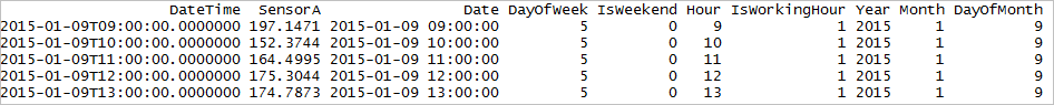
A date + time is represented in R as an object of class POSIXct. Once we convert the DateTime column into POSIXct, we can easily extract the parts of the datatime.

data$Date <- as.POSIXct(data$Date, "%Y-%m-%dT%H:%M:%S", tz="UTC")

data$DayOfWeek <- as.numeric(format(data$Date, "%u"))
data$IsWeekend <- ifelse (data$DayOfWeek>5, 1, 0)
data$Hour <- as.numeric(format(data$Date, "%H"))
data$IsWorkingHour <- ifelse (data$Hour>=9 & data$Hour<=17, 1, 0)
data$Year <- as.numeric(format(data$Date, "%Y"))
data$Month <- as.numeric(format(data$Date, "%m"))
data$DayOfMonth <- as.numeric(format(data$Date, "%d"))
tail(data, 5)

3. Trend pattern

In Python, we can use shift function to extract the features for representing the trend pattern in a time-series dataset. In R, a similar function is slide provided by DataCombine library.

data <- slide(data, Var = "SensorA", slideBy = -1:-7, 
      NewVar=c('SensorA_lag_1h', 'SensorA_lag_2h', 'SensorA_lag_3h', 'SensorA_lag_4h',
               'SensorA_lag_5h', 'SensorA_lag_6h', 'SensorA_lag_7h')
               )                                 
tail(data, 5)

We can the output as:

• Machine Learning / Data Mining
• Python/R