Context: Some trading ideas often pop into my mind unexpectedly, but most of the time I am too lazy to investigate them further. The root cause of this “laziness” is not the effort required to explore the idea itself, but rather the amount of pre-work needed before I can actually start working on it. Collecting data, building features, aligning timestamps, defining market regimes, calculating forward returns, and setting up the analysis framework can often take far more time than the research itself. One of the reasons I built QuantFlow was to reduce this friction.

This post walks through a real-world use case: systematically detecting trading opportunities from market lead-lag relationships using QuantFlow’s behaviour profiler. We’ll cover the methodology, the configuration, and what the data actually says across a diverse set of U.S. equity pairs.

Most quant research asks: “If condition X occurs, what happens to stock Y?” That’s single-symbol behavioural profiling — and it works. But markets aren’t isolated. NVDA moves, and AMD follows. MSTR breaks out, and COIN hasn’t reacted yet. QQQ sells off, and RKLB is about to catch down.

These lead-lag relationships are some of the most persistent edges in equity markets — but they’re notoriously hard to measure systematically. Most attempts fail because they rely on simple correlations rather than conditional, time-aligned, regime-aware profiling.

QuantFlow’s Behaviour Profiler now has a dedicated lead-lag mode. Here’s how it works, what it found across a diverse set of U.S. equity pairs, and why the results surprised us.

The Core Idea: Conditional Lead-Lag, Not Correlation

A naive approach:

corr(leader_ret_t, follower_ret_{t+lag})

This tells you nothing useful. It averages across all market conditions, all leader behaviours, all volatility regimes. You get a single number — usually near zero — and walk away concluding “no lead-lag exists.”

The right question isn’t “does QQQ predict NVDA?” It’s:

“When QQQ drops more than 0.5% below VWAP with a volume spike, and NVDA hasn’t moved yet, what is NVDA’s expected return over the next 15 minutes — and is it consistent across months and market regimes?”

This is conditional lead-lag profiling. The dimensions are:

leader_symbol × follower_symbol × condition × horizon × market_regime

How QuantFlow Measures Lead-Lag

The QuantFlow behaviour profiler is configured declaratively in the project YAML file, quantflow_project.yml. Here’s the configuration we used:

behaviour_profiler:
  enabled: true
  output_schema: eda
  regular_hours_only: true
  volume_z_threshold: 2.0
  target_event_count: 1000
  lead_lag:
    enabled: true
    patterns:
      - "ll_leader_momentum_up_5m"
      - "ll_leader_momentum_down_5m"
      - "ll_leader_momentum_volume"
      - "ll_leader_breakout_catchup"
      - "ll_leader_breakout_catchdown"
      - "ll_leader_large_move_gap_up"
      - "ll_leader_large_move_gap_down"
      - "ll_beta_adjusted_gap"
      - "ll_leader_volume_follower_quiet"
    pairs:
      - {leader: "QQQ",  follower: "NVDA"}
      - {leader: "QQQ",  follower: "AMD"}
      - {leader: "QQQ",  follower: "PLTR"}
      - {leader: "QQQ",  follower: "RKLB"}
      - {leader: "SPY",  follower: "TSLA"}
      - {leader: "SPY",  follower: "AAPL"}
      - {leader: "NVDA", follower: "AMD"}
      - {leader: "NVDA", follower: "MU"}
      - {leader: "NVDA", follower: "SMCI"}
      - {leader: "MSTR", follower: "COIN"}

Once configured, the profiler runs a fully automated pipeline — data loading, feature engineering, timestamp alignment, condition evaluation, forward-return measurement, and layered aggregation — writing six output tables:

lead_lag_pattern_daily
lead_lag_pattern_monthly
lead_lag_pattern_quarterly
lead_lag_pattern_yearly
lead_lag_pattern_summary
lead_lag_regime_summary

Here’s what happens under the hood.

Step 1: Build Features for Both Symbols

Leader and follower each get the full feature treatment — 1-minute OHLCV → log returns, rolling volatility, VWAP, breakout flags, streak detection, pattern flags, and market regime labels (6 categories: risk_on/off × low/normal/high vol).

Step 2: Time-Align and Compute Relative Metrics

Leader and follower features are inner-joined on datetime. Three lead-lag-specific metrics are computed:

Rolling Beta (30-bar window):

β₃₀ = Cov(leader_ret₁ₘ, follower_ret₁ₘ) / Var(leader_ret₁ₘ)

Measures how much the follower typically moves per unit of leader movement.

Expected Follower Move:

expected_move = β₃₀ × leader_ret₅ₘ

Lag Gap:

lag_gap = expected_move − follower_ret₅ₘ

This is the key metric. A positive lag_gap means the leader has moved in a way that implies the follower should have moved more, but hasn’t yet. The gap represents potential catch-up (or catch-down).

Step 3: Define Lead-Lag Conditions

Nine boolean conditions detect actionable lead-lag moments. They’re not generic “leader moved” signals — each requires a specific combination of leader behaviour and follower state:

Each condition is evaluated at every 1-minute bar. When true, we record the follower’s future return at 5, 15, and 30-minute horizons.

Step 4: Layer the Aggregation

Raw events → daily → monthly → full-sample summary. This layered approach prevents the trap of treating 500,000 correlated 1-minute observations as independent samples.

Daily level: group by (leader, follower, date, condition, horizon, regime). Metrics per day: event count, mean/median/std return, win rate, avg lag gap, avg beta.

Monthly level: group by (leader, follower, month, condition, horizon, regime). Metrics: monthly event count, monthly mean return, positive day ratio.

Full-sample summary — three key metrics are computed from the monthly aggregation:

monthly_t_stat  = mean_monthly_effect / (std_monthly_effect / √active_months)
sample_weight   = min(1.0, ln(1 + total_events) / ln(1 + target_event_count))
behavior_score  = median_monthly_effect × positive_month_ratio × sample_weight

Each serves a different purpose:

• monthly_t_stat — a t-test on monthly mean returns. Values > 2 suggest the effect is statistically meaningful, not random noise. It answers: “is this pattern’s month-to-month consistency distinguishable from zero?”
• sample_weight — a log-scaled penalty for low event counts. Patterns with fewer than the target_event_count (default 1,000) are penalized proportionally. A pattern with 500 events gets weight ≈ 0.90; 50 events gets ≈ 0.57. It answers: “do we have enough data to trust this?”
• behavior_score — the composite ranking metric, which multiplies three factors:

A behavior_score of +0.001 means the follower’s expected future return is ~+0.1% per qualifying event, consistently positive across months, with sufficient sample.

What We Found

The experiment covered multiple leader→follower pairs across 5 years of US equity data (2020–2025), with market regime labels derived from SPY’s daily trend and realized volatility.

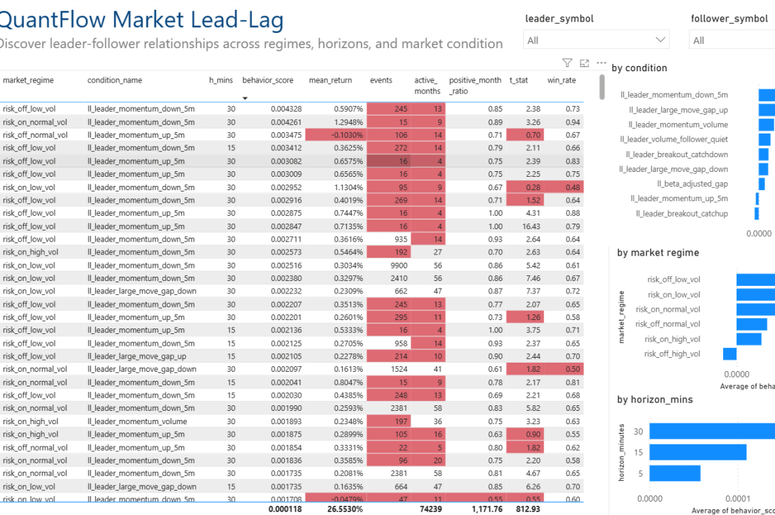
To support the analysis, a Power BI dashboard was created with the table of key metrics and dimension slicers for exploring the data interactively.

The tables are ranked by behavior_score from high to low — but raw ranking by score alone can be misleading. A pattern with a small number of events and a high mean return can generate an inflated score that collapses with more data. To avoid this, we apply a sample-quality filter before ranking. The thresholds below are suggested starting points — adjust them based on your data frequency and tolerance for false positives. Patterns that fail any of these filters are highlighted.

active_months        >= 24       (at least 2 years of data)
total_events         >= 500      (enough observations)
positive_month_ratio >= 0.60     (majority of months positive)
monthly_t_stat       >= 2        (statistically meaningful)
grand_mean_return    >  0        (positive expected value)

From the top performers that pass all filter, several potentially usable observations emerge.

Finding 1: NVDA → AMD Is the Strongest Pair

NVDA → AMD | leader_momentum_down_5m | 30m horizon | risk_on_low_vol
Active months:      56
Total events:       2,410
Positive months:    85.7% of months profitable
Monthly t-stat:     7.46
Grand mean return:  +0.33% per event

A monthly t-stat of 7.46 is exceptionally high for 1-minute event data. The effect persists across regimes too — risk_on_normal_vol shows t-stat 5.82 with 82.8% positive months. This isn’t a one-regime fluke.

Potential Interpretation: When NVDA drops meaningfully and AMD hasn’t fully followed down yet, AMD catches up with high consistency. This makes intuitive sense — both are in the semiconductor supply chain, NVDA is the bellwether, and bad news propagates through the sector with a predictable lag.

Finding 2: MSTR → COIN Is the Crypto Proxy Lead-Lag

MSTR → COIN | leader_momentum_down_5m | 30m | risk_on_low_vol
Total events:       9,900
Positive months:    85.7%
Monthly t-stat:     5.42

Potential Interpretation: MSTR acts as a leveraged Bitcoin proxy — it tends to move before COIN, the crypto exchange. When MSTR drops in a low-vol risk-on environment, COIN follows with 85%+ monthly consistency over nearly 10,000 events.This effect also holds in other regime:

This pair has also the most events of any pair, making it the most statistically robust lead-lag channel — and the high event count means practical signal frequency, not just theoretical edge.

Finding 3: The Downside Dominates

Across all pairs tested, leader_momentum_down_5m was the #1 condition in nearly every case. leader_momentum_up_5m rarely appeared in the top rankings.

This reveals a robust asymmetry: bad news propagates faster and more predictably than good news. When a leader drops, followers drop with high consistency. When a leader merely rises, followers don’t reliably follow — the signal is noisier.

However, this doesn’t mean upside lead-lag doesn’t exist. Conditions like leader_large_move_gap_up — which requires both a large leader up-move and a meaningful lag gap (follower hasn’t caught up yet) — do produce positive, stable signals for some pairs. The distinction matters: unconditional leader upside is weak; conditional upside (large move + follower lagging) can work. The strongest signals are still directional shorts when the leader breaks down, but there are long-side opportunities for traders who add the right filters.

Finding 4: Sector Lead-Lag Beats Index Lead-Lag

The strongest pairs are all intra-sector:

The weak pairs? QQQ → NVDA, SPY → TSLA. Despite being the most “obvious” pairs, they show the weakest statistical evidence. QQQ and NVDA are synchronous, not lead-lag — they move together within the same minute.

This is the most actionable finding: don’t look for lead-lag in index→mega-cap pairs — look within the supply chain.

Finding 5: Small-Cap Followers Are Regime-Dependent

QQQ → RKLB works in risk_off_high_vol (t-stat 2.08, 60% positive months) but falls apart in risk_on_high_vol.

QQQ → PLTR shows the same pattern — strong in risk-on (t-stat 2.63), dead in risk-off (t-stat 0.65).

Small-cap, high-beta followers like RKLB, PLTR, and SOUN don’t offer “always-on” lead-lag alpha. They offer regime alpha — tradable only when the market environment is right. This is where the regime dimension pays for itself.

Finding 6: Volume Is Better as a Filter Than a Trigger

Volume-based conditions (leader_momentum_volume, leader_volume_follower_quiet) fire far fewer events than price-based conditions. Their sample sizes are 10–20× smaller. This means they’re less useful as primary signals for systematic strategies.

But they can serve as confirmation filters: a price-based signal that coincides with a volume spike is stronger than one without. The volume dimension says “this move is real flow, not noise.”

What This Means for Strategy Research

The lead-lag profiler is a discovery engine, not a trading system. It answers: which pairs, under which conditions, produce stable follower reactions?

From the pairs tested, the actionable paths are:

1. NVDA → AMD: The strongest semi lead-lag. Short AMD when NVDA breaks down in low/normal vol regimes. 56 active months with 85%+ consistency.
2. MSTR → COIN: The highest-volume crypto proxy channel. 30k+ events. Works across multiple regimes. Best candidate for systematic execution.
3. NVDA → MU / SMCI: Weaker but still significant. Good for diversification — different follower, same leader logic.
4. QQQ → RKLB / PLTR: Regime-dependent. Only tradeable with a market regime filter active. Don’t run these naked.
5. QQQ → NVDA / SPY → TSLA: Skip. These are synchronous pairs, not lead-lag. The statistical evidence isn’t there.

The key insight: sector lead-lag is real, measurable, and regime-dependent. Index lead-lag is mostly noise. The pairs that look the most obvious are often the weakest — and the pairs hiding in plain sight within the supply chain are the ones worth trading.

• *Financial Data Engineering
• *QuantFlow