
The concept of “capped and floored floating-rate bonds” is covered in Section 9, Module 3 of the CFA Fixed Income curriculum. Compared to fixed-rate bonds, floating-rate bonds have distinct features that make their valuation and pricing more complex. In this blog post, I will begin by discussing the key features of floating-rate bonds and then demonstrate how to price these bonds with cap and floor limits using the QuantLib library.
Floating-Rate Bonds
Floating-rate bonds are a type of fixed-income instrument with an interest rate that is periodically adjusted based on a reference rate, such as LIBOR or SOFR, typically on a quarterly or semi-annual basis. The coupon of a floating-rate bond consists of two components: the market reference rate (MRR) and a fixed spread. For example, a bond might pay a coupon of ‘LIBOR + 2%’, where LIBOR is the reference rate and 2% is the fixed spread representing the issuer specific risks.
This periodic adjustment causes uncertainty in the bond’s cash flows, as the coupon rate fluctuates with changes in market interest rates. While this structure offers bondholders the potential for higher returns in rising rate environments, it also introduces interest rate risk. Both the issuer and the investor face uncertainty, as the coupon payments can vary throughout the life of the bond.
Capped and Floored Floating-Rate Bonds
To manage interest rate fluctuation risk, a cap (upper limit) or a floor (lower limit) can be applied to the coupon rate. In the case of a capped floating-rate bond, the coupon rate cannot exceed the specified cap, even if the reference rate rises. This benefits the issuer by limiting the coupon payments. For example, a capped bond might have a coupon rate of ‘LIBOR + 2%’ with a cap of 5%. If LIBOR exceeds 3%, the coupon rate will be limited to 5%. To compensate bondholders for the potential loss of returns when the reference rate exceeds the cap, they are typically offered a slightly higher spread.
On the other hand, a floored floating-rate bond ensures that the coupon rate cannot fall below the specified floor rate. This feature protects bondholders if interest rates drop significantly. Additionally, a floating-rate bond can have both cap and floor limits simultaneously, providing a balance of protection for both the issuer and the investor.
QuantLib FloatingRateCouponPricer
The primary distinction between a fixed-rate bond and a floating-rate bond lies in the uncertainty of future coupon payments. Pricing a fixed-rate bond is relatively straightforward due to its predictable cash flows. In contrast, pricing a floating-rate bond involves accounting for the uncertainty of future cash flows, which introduces additional complexity in modelling the dynamics of the coupon rate.
The core functionalities for pricing floating-rate bonds are encapsulated in the FloatingRateCouponPricer base class and the BlackIborCouponPricer inherited from it is one of the primary pricers used for pricing capped and floored floating-rate bonds. The inclusion of ‘Black’ in its name suggests that this pricer utilizes an approach derived from the Black model. A capped or floored floating-rate bond can be viewed as having an option-like feature on the reference interest rate. As the CFA curriculum explains:
Value of capped floater = value of straight bond – value of embedded cap
Value of floored floater = value of straight bond + value of embedded floor
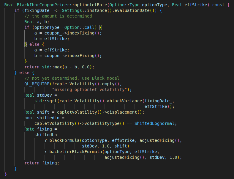
The BlackIborCouponPricer implements the optionletRate method for calculating the value of embedded options.
The BlackIborCouponPricer implements the three core methods, swapletRate, capletRate, and floorletRate, with the interface defined by the FloatingRateCouponPricer for external accesses.

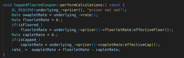
The CappedFlooredCoupon class fetches the values of those three methods and calculate the rate of the bond where the coupons attached to.
An Example
Here is a complete example I created to demonstrate the pricing of capped and floored floating-rate bonds using the QuantLib library. The full version of the code can be found at the bottom of this page.
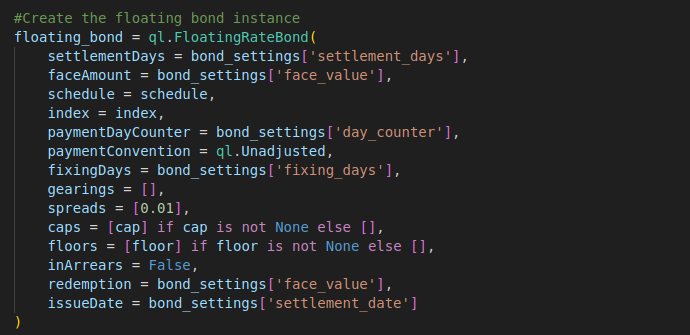
I have encapsulate the core code into the create_floating_rate_bond function, which create a FloatingRateBond instance (with some sample settings, such as bond features, schedule, cap and floor, spread etc.)
Here is the code for creating and set the BlackIborCouponPricer instance.

Full Code – QuantLib
import QuantLib as ql
import matplotlib.pyplot as plt

# Function to create floating rate bond instance
def create_floating_rate_bond(bond_settings, index,
        discounting_term_structure, volatility, cap, floor):

    #Define the bond payment schedule
    schedule = ql.Schedule(
        bond_settings['settlement_date'],
        bond_settings['maturity_date'],
        ql.Period(bond_settings['payment_freq']),
        bond_settings['calendar'],
        ql.Unadjusted,
        ql.Unadjusted,
        ql.DateGeneration.Backward,
        False
    )

    #Create the floating bond instance
    floating_bond = ql.FloatingRateBond(
        settlementDays = bond_settings['settlement_days'],
        faceAmount = bond_settings['face_value'],
        schedule = schedule,
        index = index,
        paymentDayCounter = bond_settings['day_counter'],
        paymentConvention = ql.Unadjusted,
        fixingDays = bond_settings['fixing_days'],
        gearings = [],
        spreads = [0.01],
        caps = [cap] if cap is not None else [],
        floors = [floor] if floor is not None else [],
        inArrears = False,
        redemption = bond_settings['face_value'],
        issueDate = bond_settings['settlement_date']
    )

    # set pricing engine
    engine = ql.DiscountingBondEngine(discounting_term_structure)
    floating_bond.setPricingEngine(engine)

    # set coupon pricers
    pricer = ql.BlackIborCouponPricer()
    vol = ql.ConstantOptionletVolatility(
        bond_settings['settlement_days'],
        bond_settings['calendar'],
        ql.Unadjusted,
        volatility,
        bond_settings['day_counter']
    )
    option_vol_handle = ql.OptionletVolatilityStructureHandle(vol)
    pricer.setCapletVolatility(option_vol_handle)
    ql.setCouponPricer(floating_bond.cashflows(), pricer)

    return floating_bond

# Utility function for drawing line chart
def draw_chart(title, x_data, x_title, y1, y1_title, y2_data=None, y2_title=None, x_invert=False):

    fig, ax1 = plt.subplots(figsize=(8, 4))

    for y in y1:
        ax1.plot(x_data, y[0], label=y[1], color=y[2], linewidth=2)
    ax1.set_xlabel(x_title, fontsize=12)
    ax1.set_ylabel(y1_title, color='b', fontsize=12)
    ax1.tick_params(axis='y', labelcolor='b')
    ax1.grid(True)

    if y2_data is not None:
        ax2 = ax1.twinx()
        ax2.plot(x_data, y2_data, label=y2_title, color='red', linewidth=2)
        ax2.set_ylabel(y2_title, color='red', fontsize=12)
        ax2.tick_params(axis='y', labelcolor='red')

    if x_invert:
        ax=plt.gca()
        ax.invert_xaxis()
    plt.ylim()
    plt.ylim()
    plt.legend()
    plt.title(title, fontsize=16)
    fig.tight_layout()
    plt.show()


# Set evaluation date for QuantLib
today = ql.Date(23, 12, 2024)
ql.Settings.instance().evaluationDate = today

# Market rate and volatility
rate = 0.03
volatility = 0.05

# Define the bond features
bond_settings = {
    'calendar': ql.UnitedStates(ql.UnitedStates.NYSE),
    'day_counter': ql.Actual360(),
    'settlement_days': 3,
    'settlement_date': ql.Date(1, 1, 2025),
    'maturity_date': ql.Date(1, 1, 2033),
    'fixing_days': 2,
    'payment_freq': ql.Quarterly,
    'coupon_rate': 0.02,
    'face_value': 100,
}

# Spot rates for pricing the bond
spot_rates = [
    (ql.Date(15, 12, 2024), 0.02),
    (ql.Date(15, 12, 2025), 0.0325),
    (ql.Date(15, 12, 2026), 0.034),
    (ql.Date(15, 12, 2027), 0.038),
    (ql.Date(15, 12, 2028), 0.04),
    (ql.Date(15, 12, 2029), 0.042),
    (ql.Date(15, 12, 2030), 0.043),
    (ql.Date(15, 12, 2031), 0.0465),
    (ql.Date(15, 12, 2032), 0.047),
    (ql.Date(15, 12, 2033), 0.0468)
]
spot_curve = ql.ZeroCurve([rate[0] for rate in spot_rates],
                                      [rate[1] for rate in spot_rates], ql.Actual360())

# create term structure for discounting the bond cash flows
discounting_term_structure = ql.RelinkableYieldTermStructureHandle(spot_curve)

# create reference index
index = ql.Euribor3M(
    ql.RelinkableYieldTermStructureHandle(spot_curve)
)

# create capped and floored floater and pricing based on a range of
# different cap or floor rate
cap_floors = [0.01, 0.02, 0.03, 0.04, 0.05, 0.06, 0.07, 0.08, 0.09]
capped_bond_prices = []
floored_bond_prices = []

# use quote and quote handle to enable auto update
rate_level = ql.SimpleQuote(0)
rate_level_handle = ql.QuoteHandle(rate_level)

# loop through cap/floor rates to calulate bond prices for each rate
for i in cap_floors:
    rate_level = i

    capped_floater = create_floating_rate_bond(bond_settings, index,
        discounting_term_structure, volatility, rate_level, None)
    capped_bond_prices.append(capped_floater.NPV())

    floored_floater = create_floating_rate_bond(bond_settings, index,
        discounting_term_structure, volatility, None, rate_level)
    floored_bond_prices.append(floored_floater.NPV())

draw_chart('', cap_floors, 'Cap/Floor Rate',
           [(capped_bond_prices, 'Capped Bond', 'blue'),
            (floored_bond_prices, 'Floored Bond', 'orange')],
           'Price')
