The interest rate term structure models are discussed in the CFA curriculum, Fixed Income, Module 2, Section 8. This section focuses on understanding how interest rates evolve over time, with models used to explain and predict the term structure of interest rates. Modeling the future path of interest rates is critical for a wide range of valuation and analysis in the world of fixed-income investment. It is an essential input when using quantitative libraries for valuing fixed-income instruments.

Term structure models employ stochastic processes to capture the behaviour of interest rates over time. These models consist of two fundamental elements: a drift component and a stochastic component. Here is the general form of the process for a one-factor short rate model.

The drift term (θ) reflects the expected, deterministic direction in which interest rates are likely to move, influenced by factors such as economic trends, inflation, and central bank policies. In contrast, the stochastic term (σ) introduces randomness and volatility, accounting for unexpected changes in the market driven by external factors and market sentiment.

Four term structure models are covered in the CFA curriculum: two arbitrage-free models, the Ho-Lee model and the Kalotay-Williams-Fabozzi model, and two equilibrium models, the Cox-Ingersoll-Ross (CIR) model and the Vasicek model. In this blog post, I will simulate these models in Python, based on the algorithms provided in the CFA curriculum.

Arbitrage-Free Models

Arbitrage-free models ensure that there are no arbitrage opportunities in the market by aligning the pricing of instruments with observed market data. They are considered as the accurate modelling with respect to the observed term structure, which leads it to be widely used in practice. The main weakness of this class of models is the limited ability to interpret the underlying economic forces that drive interest rates.

Ho-Lee Model

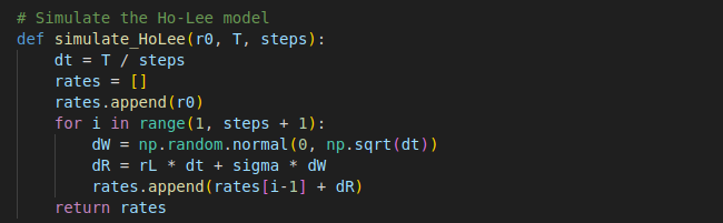
The Ho-Lee model is one of the simplest term structure models. Both the drift term (θ) and the volatility term (σ) are constant in the model, meaning it ignores time-varying volatilies.

Due to its constant drift and volatility, the model requires fewer parameters and can be calibrated using market data efficiently. Here is the Python code modeling the Ho-Lee process. The calibration of the model terms is not the focus of this blog post. For the purpose of this demonstration, we assume that the drift term and volatility term have already been fixed based on market data.

Kalotay-Williams-Fabozzi Model

The Kalotay-Williams-Fabozzi Model is an enhanced version of the Ho-Lee model, which assumes the short rate is distributed lognormally.

The logarithmic transformation of the Ho-Lee model prevents the rate from becoming negative, which is relatively more aligned with the real-world situations. In addition, the logarithmic transformation helps stabilise large changes in interest rates, making this formulation more stable in extreme market conditions.

Equilibrium Models

While arbitrage-free models focus on market consistency, equilibrium models are based on economic fundamentals, which are driven by underlying factors such as economic growth, inflation expectations, and other macroeconomic variables. In equilibrium models, interest rates reflects the balance between these economic factors, adjusting over time to align with long-term economic conditions.

Cox-Ingersoll-Ross (CIR) Model

The Cox-Ingersoll-Ross (CIR) model is widely regarded as one of the most effective models in practice for modeling interest rate dynamics. Here is the formula for CIR model.

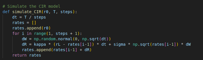
One of the main strengths of CIR is its ability to capture mean reversion, a key characteristic of interest rates in the real world, where rates tend to return to a long-term average over time. From the formula above we can see, the drift term consists of three components: current rate, r(t); the long-term average rate, u; and the rate reverting speed to its mean (θ), which representing the mean reversion pattern in the rate movements.

For the volatility term, it is proportional to the square root of the interest rate, r(t), which ensures the short term interest rate to be positive and also reflects the real-world market behaviour where volatility tends to decrease when rates are low.

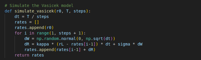
Vasicek Model

Similar to the CIR model, the Vasicek model reflects the mean reversion market behaviour. As the formula below shows, the drift term of Vasicek model is the same as the CIR model’s. The main difference between these two models is that the Vasicek model assumes constant volatility, which can theoretically result in negative interest rates

We can run the simulation of the four processes above across a period of time to have the simulated interest rate paths. The full code for the simulation and visualisation can be found below.

Full Code – Python

import numpy as np
import matplotlib.pyplot as plt

# utility function for drawing line chart
def draw_chart(title, x_data, x_title, y1, y1_title, y2_data=None, y2_title=None, x_invert=False):

    fig, ax1 = plt.subplots(figsize=(8, 4))
    
    for y in y1:
        ax1.plot(x_data, y[0], label=y[1], color=y[2], linewidth=2)
    ax1.set_xlabel(x_title, fontsize=12)
    ax1.set_ylabel(y1_title, color='b', fontsize=12)
    ax1.tick_params(axis='y', labelcolor='b')
    ax1.grid(True)

    if y2_data is not None:
        ax2 = ax1.twinx()
        ax2.plot(x_data, y2_data, label=y2_title, color='red', linewidth=2)
        ax2.set_ylabel(y2_title, color='red', fontsize=12)
        ax2.tick_params(axis='y', labelcolor='red')

    if x_invert:
        ax=plt.gca()
        ax.invert_xaxis()
    plt.legend()
    plt.title(title, fontsize=16)
    fig.tight_layout()
    plt.show()

# Simulate the Ho-Lee model
def simulate_HoLee(r0, T, steps):
    dt = T / steps
    rates = []
    rates.append(r0)
    for i in range(1, steps + 1):
        dW = np.random.normal(0, np.sqrt(dt))
        dR = rL * dt + sigma * dW
        rates.append(rates[i-1] + dR)
    return rates

# Simulate the Vasicek model
def simulate_vasicek(r0, T, steps):
    dt = T / steps
    rates = []
    rates.append(r0)
    for i in range(1, steps + 1):
        dW = np.random.normal(0, np.sqrt(dt))
        dR = kappa * (rL - rates[i-1]) * dt + sigma * dW
        rates.append(rates[i-1] + dR)
    return rates

# Simulate the CIR model
def simulate_CIR(r0, T, steps):
    dt = T / steps
    rates = []
    rates.append(r0)
    for i in range(1, steps + 1):
        dW = np.random.normal(0, np.sqrt(dt))
        dR = kappa * (rL - rates[i-1]) * dt + sigma * np.sqrt(rates[i-1]) * dW
        rates.append(rates[i-1] + dR)
    return rates

# Simulate the Kalotay-Williams-Fabozzi model
def simulate_KWF(r0, T, steps):
    dt = T / steps
    log_rates = [] 
    log_rates.append(np.log(r0))
    for i in range(1, steps + 1):
        dW = np.random.normal(0, np.sqrt(dt))
        dR = rL * dt + sigma * dW
        log_rates.append(log_rates[i-1] + dR)
    
    return np.exp(log_rates)


r0 = 0.05
rL = 0.05
kappa = 0.05 
sigma = 0.05
T = 5
steps = 1000 

X = np.linspace(0, T, steps + 1)
y_vasicek = simulate_vasicek(r0, T, steps)
y_CIR = simulate_CIR(r0, T, steps)
y_KWF = simulate_KWF(r0, T, steps)
y_HoLee = simulate_HoLee(r0, T, steps)

draw_chart("Term Structure Models", X, "Time",
           [(y_HoLee, "Ho Lee", "blue"),
            (y_vasicek, "Vasicek", "orange"),
            (y_CIR, "CIR", "brown"),
            (y_KWF, "KWF", "green")
            ], "Rate")

• Coding towards CFA