
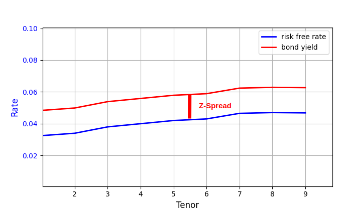
The Z-spread is an important metric for analysing the yield premium on a bond. It measures the constant spread over the benchmark yield curve, typically a risk-free curve, representing the additional credit or liquidity risks associated with the bond.
Key features of Z-spread
- Risk-free benchmark – the Z-spread is measured with a risk-free curve as benchmark so that it reflects the credit risk, liquidity risk, and other factors embedded in a bond relative to a risk-free investment.
- Constant Spread – the Z-spread is added uniformly to each point along the risk-free curve, leading to a parallel level-shift of the curve.
- No Volatility Adjustment – the letter Z refers to Zero-volatility, meaning that Z-spread is calculated under the assumption of the constant or zero volatility.
The Z-spread is normally determined by solving the equation where the bond price, calculated by discounting the bond’s future cash flows, equals to the observed market price.
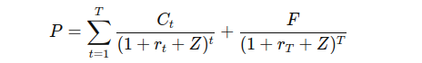
The core task here is to determine the constant Z in the formula. Unfortunately, there is not a simple and accurate closed-form solution for solving the Z, instead, the Z is calculated through the iterative “trial-and-error”. We can use the scipy.optimize.brentq method, or the built-in brent method offered by QuantLib, for this task.
This is the function I created for demonstrating the calculation of Z-spread using QuantLib. The full version ready-go run code is attached at bottom of this page.

Prior to calling the function, we need create a QuantLib Bond instance. We can reuse the create_fixed_rate_bond function we created in the previous blog post.
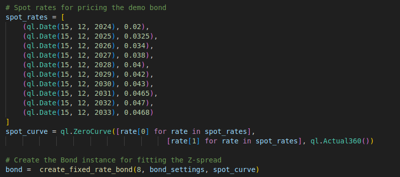
This Bond instance will be used to calculate the present value, which will be compared to the observed market price. The z_spread_func is the objective function for updating the curve by adding the “guess” z_spread over the spot rates.

A Brent solver instance is created for solving the z_spread_func objective function for the target z_spread.

Full Code – QuantLib
import QuantLib as ql
import matplotlib.pyplot as plt

# Function to calculate the Z-spread using the Brent solver
def calculate_z_spread(bond, market_price, spot_rates, day_counter):

    # The root-finding function for finding spread that makes the bond
    # price close to market price
    def z_spread_func(z_spread):
        curve = ql.ZeroCurve([rate[0] for rate in spot_rates],
                                      [rate[1] + z_spread for rate in spot_rates],
                                      day_counter)
        z_spread_handle = ql.YieldTermStructureHandle(curve)
        bond.setPricingEngine(ql.DiscountingBondEngine(z_spread_handle))
        return bond.NPV() - market_price

    # Create and configure the Brent solver
    accuracy = 1e-5
    guess = 0.005
    min = 1e-6
    max = 1
    solver = ql.Brent()
    solver.setMaxEvaluations(100)

    # Solve the spread
    z_spread = solver.solve(z_spread_func, accuracy, guess, min, max)

    return z_spread

# Function to create fixed rate bond instance
def create_fixed_rate_bond(maturity, bond_settings, spot_curve):

    #Load the bond attributes
    calendar = bond_settings['calendar']
    day_counter = bond_settings['day_counter']
    settlement_days = bond_settings['settlement_days']
    payment_freq = bond_settings['payment_freq']
    face_value = bond_settings['face_value']
    coupon_rate = bond_settings['coupon_rate']
    settlement_date = calendar.advance(today, ql.Period(settlement_days, ql.Days))

    #Define the bond cashflow schedule
    schedule_bond = ql.Schedule(
        settlement_date,
        calendar.advance(settlement_date, ql.Period(maturity, ql.Years)),
        ql.Period(payment_freq),
        calendar,
        ql.Unadjusted,
        ql.Unadjusted,
        ql.DateGeneration.Backward,
        False
    )

    #Create fixed rate bond
    bond = ql.FixedRateBond(settlement_days, face_value, schedule_bond,
                                [coupon_rate], day_counter)

    bond_engine = ql.DiscountingBondEngine(ql.YieldTermStructureHandle(spot_curve))
    bond.setPricingEngine(bond_engine)

    return bond

# Utility function for drawing line chart
def draw_chart(title, x_data, x_title, y1, y1_title, y2_data=None, y2_title=None, x_invert=False):

    fig, ax1 = plt.subplots(figsize=(8, 4))

    for y in y1:
        ax1.plot(x_data, y[0], label=y[1], color=y[2], linewidth=2)
    ax1.set_xlabel(x_title, fontsize=12)
    ax1.set_ylabel(y1_title, color='b', fontsize=12)
    ax1.tick_params(axis='y', labelcolor='b')
    ax1.grid(True)

    if y2_data is not None:
        ax2 = ax1.twinx()
        ax2.plot(x_data, y2_data, label=y2_title, color='red', linewidth=2)
        ax2.set_ylabel(y2_title, color='red', fontsize=12)
        ax2.tick_params(axis='y', labelcolor='red')

    if x_invert:
        ax=plt.gca()
        ax.invert_xaxis()
    plt.ylim(bottom=0)
    plt.ylim(top=0.1)
    plt.legend()
    plt.title(title, fontsize=16)
    fig.tight_layout()
    plt.show()


# Set evaluation date for QuantLib
today = ql.Date(23, 12, 2024)
ql.Settings.instance().evaluationDate = today

# Define the settings of the fixed bonds for riding the yield curve
bond_settings = {
    'calendar': ql.UnitedStates(ql.UnitedStates.NYSE),
    'day_counter': ql.Actual360(),
    'settlement_days': 2,
    'payment_freq': ql.Annual,
    'coupon_rate': 0.05,
    'face_value': 100
}

# Spot rates for pricing the demo bond
spot_rates = [
    (ql.Date(15, 12, 2024), 0.02),
    (ql.Date(15, 12, 2025), 0.0325),
    (ql.Date(15, 12, 2026), 0.034),
    (ql.Date(15, 12, 2027), 0.038),
    (ql.Date(15, 12, 2028), 0.04),
    (ql.Date(15, 12, 2029), 0.042),
    (ql.Date(15, 12, 2030), 0.043),
    (ql.Date(15, 12, 2031), 0.0465),
    (ql.Date(15, 12, 2032), 0.047),
    (ql.Date(15, 12, 2033), 0.0468)
]
spot_curve = ql.ZeroCurve([rate[0] for rate in spot_rates],
                                      [rate[1] for rate in spot_rates], ql.Actual360())

# Create the Bond instance for fitting the Z-spread
bond =  create_fixed_rate_bond(8, bond_settings, spot_curve)

# Calculate the Z-spread
z_spread = calculate_z_spread(bond, 97, spot_rates, ql.Actual360())
print(z_spread)


# Plot the z-curve
tenors = list(range(1, 9))
full_spot_rates = [spot_curve.zeroRate(bond_settings["calendar"].advance(today, ql.Period(i, ql.Years)),
                                    ql.Actual360(), ql.Continuous
                                ).rate() for i in tenors
            ]
bond_rates = [r + z_spread for r in full_spot_rates]
draw_chart("", x_data=tenors, x_title="Tenor",
            y1=[
                (full_spot_rates, "risk free rate", "blue"),
                (bond_rates, "bond yield", "red")
            ], y1_title="Rate")
