
“Riding the Yield Curve” is the topic covered in the CFA Fixed Income, Module 1, Section 3, “Active Bond Portfolio Management”. In this blog post, I will simulate the approach discussed in the CFA curriculum with the support of the QuantLib library.
“Riding the Yield Curve”, also known as “Rolling Down the Yield Curve”, is a popular yield curve trading strategy. It involves going long on bonds with maturities longer than the investment horizon and shorting bonds after the investment horizon, rather than holding bonds with a maturity that matches the investment horizon. This strategy relies on two key assumptions:
- The yield curve is upward sloping
- The yield curve remains static over an investment horizon
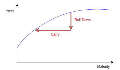
In a market condition where the yield curve slopes upward and remains relatively static over an investment horizon, as a bond approaches its maturity, it is progressively valued at lower yields and higher prices. Consequently, the bond’s price increases as it ‘rolls down’ the yield curve, which results in capital gains for the investor holding a bond with longer maturity.
The CFA curriculum breaks the total return of a fixed-rate bond into three components: coupons, interest from coupon reinvestment, and capital gains from selling the bond prior to maturity. The first two components represent the ‘Carry‘ return of the bond, which compensates the investor for the time value of money, while the last component is the ‘Roll-Down‘ return, which results from the interest rate fluctuations in the bond’s price.
In the following assumed example, there two trading options for a 3 years investment horizon:
- Long a 3 year fixed-rate bond and hold to maturity
- Long a 10 years fixed-rate Bond and short after 3 years
Let’s take a look at the result first before looking into the code details.
We created three QuantLib bond instances with the maturity of year 3, year 10 and year 7, and calling the NPV method to return the evaluated price of each. As the investment lengths for the two trading options are same, i.e. 3 years, the carry returns are some for them. Therefore, we only need to compare the price differences.

The result shows that the gains from price movement of 3 year hold-to-maturity bond is 4.67 and the gains from the curve riding option is 7.05.

Now let’s look into the code. First, we need fit the spot curve from the market rates. Here, we can reuse the fit_spot_curve_from_par function we created in the previous blog post. The full code of the function can be found at the bottom of this page.

The create_fixed_rate_bond function create a QuantLib FixedRateBond instance. An DiscountingBondEngine instance is created that uses the yield curve we just fit earlier. With the FixedRateBond instance, we can trigger the pricing with its NPV or cleanPrice methods.

Full Code – QuantLib
import QuantLib as ql

# Function to fit spot curve from a par curve using QuantLib
def fit_spot_curve_from_par(maturities, pars, bond_settings,
                                            fit_method, fit_model=None):

    # Fetch the settings of the bond instruments used for curve fitting
    calendar = bond_settings['calendar']
    day_counter = bond_settings['day_counter']
    settlement_days = bond_settings['settlement_days']
    payment_freq = bond_settings['payment_freq']
    settlement_date = calendar.advance(today,
                                       ql.Period(settlement_days, ql.Days))

    # Loop through the provided maturities and create bond helpers for each
    rate_helpers = []
    for i in range(len(maturities)):

        # Calculate maturity date by advancing settlement
        # date by the maturity period
        maturity_date = calendar.advance(settlement_date,
                    ql.Period(maturities[i], ql.Years))

        #Define the bond cashflow schedule
        schedule = ql.Schedule(
            settlement_date,
            maturity_date,
            ql.Period(payment_freq),
            calendar,
            ql.ModifiedFollowing,
            ql.ModifiedFollowing,
            ql.DateGeneration.Backward,
            False)

        #Create the fixed rate bond helper for the maturity date
        helper = ql.FixedRateBondHelper(
            ql.QuoteHandle(ql.SimpleQuote(100)),
            settlement_days,
            100.0,
            schedule,
            [pars[i]/100],
            day_counter
        )

        rate_helpers.append(helper)


    if fit_model is None:
        # fit the curve using the fit method specified through the fit_method parameter
        curve = fit_method(today, rate_helpers, day_counter)
    else:
        # The fit_model is only provided when using FittedBondDiscountCurve
        curve = fit_method(settlement_days, calendar, rate_helpers, day_counter, fit_model)

    return curve

# Function to create fixed rate bond instance
def create_fixed_rate_bond(maturity, bond_settings, spot_curve):

    #Load the bond attributes
    calendar = bond_settings['calendar']
    day_counter = bond_settings['day_counter']
    settlement_days = bond_settings['settlement_days']
    payment_freq = bond_settings['payment_freq']
    face_value = bond_settings['face_value']
    coupon_rate = bond_settings['coupon_rate']
    settlement_date = calendar.advance(today, ql.Period(settlement_days, ql.Days))

    #Define the bond cashflow schedule
    schedule_bond = ql.Schedule(
        settlement_date,
        calendar.advance(settlement_date, ql.Period(maturity, ql.Years)),
        ql.Period(payment_freq),
        calendar,
        ql.Unadjusted,
        ql.Unadjusted,
        ql.DateGeneration.Backward,
        False
    )

    #Create fixed rate bond
    bond = ql.FixedRateBond(settlement_days, face_value, schedule_bond,
                                [coupon_rate], day_counter)

    bond_engine = ql.DiscountingBondEngine(ql.YieldTermStructureHandle(spot_curve))
    bond.setPricingEngine(bond_engine)

    return bond


# Set evaluation date for QuantLib
today = ql.Date(23, 12, 2024)
ql.Settings.instance().evaluationDate = today

###########################################
#     Fit Spot Curve from Par Rates       #
###########################################

# The market par rates for fitting curve
maturities = [1, 2, 3, 5, 7, 10, 20, 30]
pars = [3, 3.3, 3.6, 4, 4.2, 4.5, 4.8, 5]

# Define the settings of the par bond for curve fitting
curve_fitting_bond_settings = {
    'calendar': ql.UnitedStates(ql.UnitedStates.NYSE),
    'day_counter': ql.Actual360(),
    'settlement_days': 2,
    'payment_freq': ql.Semiannual
}
spot_curve = fit_spot_curve_from_par(maturities, pars, curve_fitting_bond_settings,
                         ql.PiecewiseLogCubicDiscount)

###########################################
#         Price Fixed-Rate Bonds          #
###########################################

# Define the settings of the fixed bonds for riding the yield curve
bond_settings = {
    'calendar': ql.UnitedStates(ql.UnitedStates.NYSE),
    'day_counter': ql.Actual360(),
    'settlement_days': 2,
    'payment_freq': ql.Annual,
    'coupon_rate': 0.02,
    'face_value': 100
}

# 3-year bond
bond_3y = create_fixed_rate_bond(3, bond_settings, spot_curve)
price_3y = bond_3y.NPV()

# 10-year bond
bond_10y = create_fixed_rate_bond(10, bond_settings, spot_curve)
price_10y = bond_10y.NPV()

# 7-year bond
bond_7y = create_fixed_rate_bond(7, bond_settings, spot_curve)
price_7y = bond_7y.NPV()

diff_10y = price_7y - price_10y
diff_3y = 100 - price_3y

print("price gains on long 3ys bond: "+str(diff_3y))
print("price gains on long 10ys bond and hold for 3ys: "+str(diff_10y))
