In the previous blog post, we saw that the binomial model closely approximates option prices as the number of periods increases. The binomial model is known for its flexibility, intuitiveness, and fewer assumptions. So, why do we still need the Black-Scholes-Merton (BSM) model for option pricing, especially given its restrictive assumptions?

One of the main drawbacks of the binomial model is the need for recursive calculations across a multi-step lattice, which becomes computationally intensive as the number of periods increases. This makes the binomial model inefficient for many real-world financial applications.

The beauty of the BSM model lies in its closed-form solution, which offers a direct, fast, and efficient way to calculate option prices with minimal computational effort. This simplicity makes BSM highly applicable for real-world option pricing scenarios. In addition to pricing options, directness of BSM formula calculation makes it capable to derive the Greeks in real-time, which is crucial for effective risk management.

As the industry standard for option pricing, the BSM model has been thoroughly tested in both academic research and industry practice. It provides the theoretical foundation for many advanced option pricing models and derivative strategies, such as the Black model for pricing options on futures and other derivatives.

In this blog post, I will explore the BSM model, covering its assumptions, key inputs, formula, and implementation with Python and DolphinDB.

Assumptions of the BSM Model

• The price of underlying follows Geometric Brownian Motion (GBM) process, i.e., the continuously compounded return is normally distributed.
• The price of underlying is continuous.
• The underlying needs to be liquid at the market.
• Continuous trading is available.
• Short selling is allowed.
• No market frictions.
• No arbitrage opportunities avaliable.
• The options are European style.
• The continuously compounded risk-free interest rate is known and constant.
• The volatility of the return on the underlying is known and constant.
• The yields of underlying is expressed as a continuous known and constant.

Key Inputs of the BSM Model

Here is a list of the key parameters that feed into the BSM model to determine the option price. In other words, the price of an option is influenced by the following variables:

• Current underlying price (S): the underlying asset price at the option valuation time.
• Strike price (K): the price agreed for exercise at option expiration.
• Time to expiration (T): the time remaining until the option expiration.
• Risk-free interest rate (r): the interest rate of a risk-free asset.
• Volatility (σ): the standard deviation of the returns of the underlying asset.

Formula Interpretation

Here is the famous BSM formula for option pricing. This is the fundamental form, and many extensions or adaptations for more complex option pricing scenarios are derived from it.

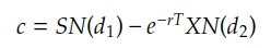
The BSM model is difficult to derive, requiring advanced mathematical tools such as stochastic calculus and Ito’s Lemma. However, once derived, the interpretation and application of the model are straightforward.

In the BSM model, the core idea behind option pricing is constructing a replicating portfolio using a combination of the underlying asset, such as stock, and a financing component, such as a risk-free bond, to replicate the option’s payoff at expiration. The value of the option can be derived from the cost of this portfolio. Taking an call option as example:

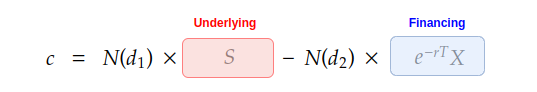
At an abstract level, a call option can be replicated by a portfolio consisting of a long position in N(d1) shares of stock and a short position in a risk-free bond with an amount proportional to N(d2). By continuously adjusting the quantities of stock and bond in the portfolio as market conditions change, we ensure that the portfolio’s value matches the option price, thereby eliminating any arbitrage opportunities. As a result, the price of the call option can be determined by the cost of the constructed portfolio.

In the BSM model, N(d1) represents the probability that the option will be in-the-money at expiration, in the form of the cumulative distribution function (CDF) of the standard normal distribution evaluated at d1. d1 represents the normalised distance between the current stock price and the strike price. Here is the formula for calculating d1:

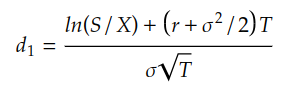
The term ln⁡(S/X) represents the relative distance between the current stock price and the strike price. When S>X, the option is ‘in-the-money,’ and when S<X, the option is ‘out-of-the-money.’ The term (r+σ^2/2)T represents how the stock price fluctuates over time, taking into account the drift rate and volatility. The term σ*sqrt(T) is used for standardisation purposes. From the formula, we can see that d1​ combines information about the stock’s price movement with the effects of time and volatility.

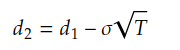
N(d2) represents the probability that the option will be exercised at expiration, which is adjusted by the present value of the strike price and the time value of money. d2​ is derived directly from d1 with adjusted by subtracting the volatility term, σ*sqrt(T)​.

The code implementation of the BSM formula is pretty simple. Here is the Python code implementation.

Full Code – Python

import numpy as np
from scipy.stats import norm

def value_option_bsm(s, k, T, r, sigma, option_type="call"):

    # Calculate d1 and d2
    d1 = (np.log(s / k) + (r + 0.5 * sigma ** 2) * T) / (sigma * np.sqrt(T))
    d2 = d1 - sigma * np.sqrt(T)

    # Calculate option price
    if option_type == "call":
        option_price = s * norm.cdf(d1) - k * np.exp(-r * T) * norm.cdf(d2)
    else:
        option_price = k * np.exp(-r * T) * norm.cdf(-d2) - s * norm.cdf(-d1)

    return option_price


s = 100
k = 100
T = 1
r = 0.05
sigma = 0.2

call_price = value_option_bsm(s, k, T, r, sigma, option_type="call")
put_price = value_option_bsm(s, k, T, r, sigma, option_type="put")

print("Call Option Price: "+str(call_price))
print("Put Option Price: "+str(put_price))

Full Code – DolphinDB

def value_option_bsm(s, k, T, r, sigma, option_type="call"){

    // Calculate d1 and d2
    d1 = (log(s / k) + (r + 0.5 * pow(sigma, 2)) * T) / (sigma * sqrt(T))
    d2 = d1 - sigma * sqrt(T)

    // Calculate option price
    if (option_type == "call")
        option_price = s * cdfNormal(0, 1, d1) - k * exp(-r * T) * cdfNormal(0, 1, d2)
    else
        option_price = k * exp(-r * T) * cdfNormal(0, 1, -d2) - s * cdfNormal(0, 1, -d1)

    return option_price
}

s = 100
k = 100
T = 1
r = 0.05
sigma = 0.2

call_price = value_option_bsm(s, k, T, r, sigma, option_type="call")
put_price = value_option_bsm(s, k, T, r, sigma, option_type="put")

print("Call Option Price: "+call_price)
print("Put Option Price: "+put_price)

• Coding towards CFA