In the previous blog post, we explored the historical approach for estimating the Equity Risk Premium (ERP). The historical approach is a widely used method that is simple to implement. However, it relies on the assumption that the future will resemble the past, which often does not hold true in financial markets. In this blog post, we will examine forward-looking approaches for estimating ERP, including the survey-based approach, the Dividend Discount Model (DDM) approach, and the macroeconomic modeling approach.

Survey-based Estimates

The survey-based approach involves gathering experts’ subjective expectations of the Equity Risk Premium (ERP). This approach is simple to implement, as it does not rely on a mathematical model. Therefore, it is more flexible and customizable for special situations. Since this approach captures current market sentiment, it is particularly useful for short-term forecasts.

On the other hand, this approach relies on subjective opinions, which can be biased and may lack consensus among experts. It is particularly prone to overreacting to recent events. In addition, there is a lack of historical data for validation.

Dividend Discount Model Estimates

The Dividend Discount Model (DDM) is a fundamental approach used to estimate the Equity Risk Premium (ERP), the required return on equity, and the intrinsic value of equity. This approach calculates the present value of expected future dividends to determine the intrinsic value of a stock. One of the most widely used DDM approaches is the Gordon Growth Model (GGM), which assumes that dividends grow at a constant rate. Below is the formula for the GGM, used to calculate the intrinsic value of a stock, where:

• g = Constant growth rate of dividends.
• D1​ = Expected dividend in the next period,
• r(e) = Required rate of return for the stock,

From the formula, after a simple transformation, we can derive the following formula for calculating the required rate of return:

From the required rate of return, we can calculate the ERP by subtracting the risk-free rate from the required rate of return. Below is the formula used to derive the ERP using the (GGM):

Here, we are going to implement an ERP calculation function in Python based on the formula above. To use this formula, we need the following parameters:

D1 – Expected dividend in the next period

This can be derived as D0 * (1 + g).

D0 – Dividend in the current period

This can be retrieved from the historical market data of a broad market equity index proxy.

V0 – Current value of the stock market

The current price of the broad market equity index proxy, such as an ETF, can be used as V0.

g – Constant dividend growth rate

This can be calculated from the dividend history of the equity index proxy.

r(f) – Risk-Free Rate

We can use the yield of a government bond, such as the 10-year US Treasury Bond, as the risk-free rate.

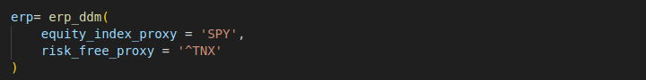
In our example here, we will use SPY (SPDR S&P 500 ETF) as the proxy for equity market and the 10-year US Treasury Bond as the proxy for risk-free rate.

We can fetch the historical price data and dividend data of SPY from a market data API, such as Yahoo Finance. Since the dividends of SPY are accounted for quarterly, we need to annualise them.

From the dividends history, we can derive the constant growth rate, g.

With the derived dividend growth rate (g), we can derive the expected dividend for the next period (D1), by using current dividend (D0) times (1 + g). Once we have fetched the market data for the current SPY price (V0) and the yield of the US Treasury Bond as the risk-free rate (r(f)​), we can calculate the ERP using the formula described above.

Macroeconomic Modelling

ERP can also be estimated using macroeconomic models that rely on forecasted economic variables to provide insights into expected equity market returns. One of these models is Grinold-Kroner decomposition or the return on equity. First, the return on equity can be from the Dividend Yield (DY) and Expected capital gain (delta-P).

As the stock price can be calculated as P/E ratio times the earning per share (EPS),

We can derive the change of the stock price is from the change of P/E ratio and the growth of EPS.

The growth of EPS (Earnings Per Share) can be expressed as the sum of expected inflation (i) and real economic growth (g), minus the percentage change in shares outstanding.

Putting all the pieces together, we can derive the formula for calculating the ERP, incorporating considerations of these macroeconomic factors.

Full Code – Python

import yfinance as yf
import numpy as np

# Fetch annualized dividend data and the latest price for a given equity index proxy.
def fetch_annualised_dividend_data(equity_index_proxy):
    
    # Fetch stock data from yfinance
    stock = yf.Ticker(equity_index_proxy)

    # Load historical dividends
    dividends = stock.dividends
    if dividends.empty:
        raise Exception(f"No dividend data avalaible.")

    # Fetch the latest stock price
    stock_info = stock.history(period="1y")
    latest_price = stock_info['Close'].iloc[-1]

    # Get annalised total dividends
    annualised_dividends = dividends.resample("Y").sum()
    
    return annualised_dividends, latest_price

# Fetch the market data as input to DDM
def fetch_market_data(equity_index_proxy, risk_free_proxy):

    # Fetch annualized dividend data and the latest price for a given equity index proxy.
    dividends, equity_index_price = fetch_annualised_dividend_data(equity_index_proxy)

    # Fetch the risk free rate (yield of the proxy debt)
    risk_free_rate_proxy = yf.Ticker(risk_free_proxy)
    risk_free_rate = risk_free_rate_proxy.history(period="1d")['Close'].iloc[-1] / 100  

    return equity_index_price, dividends, risk_free_rate

# Calculate dividend growth rate, g
def calculate_dividend_growth_rate(annualised_dividends, periods):
    
    if len(annualised_dividends) < 2:
        raise Exception(f"No sufficient dividend data avalaible.")

    # select the historical period for estimate the dividend growth
    dividends = annualised_dividends[-periods:]

    # cacluate the compound annual growth rate
    beginning_value = dividends.iloc[0]
    ending_value = dividends.iloc[-1]
    g = (ending_value / beginning_value) ** (1 / periods) - 1

    return g


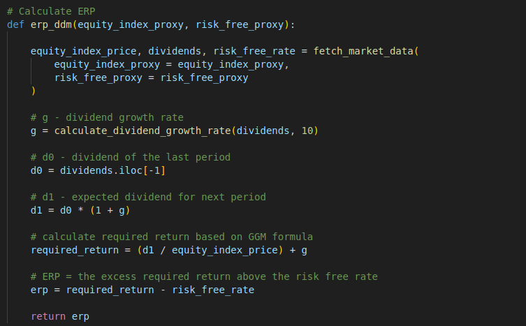
# Calculate ERP
def erp_ddm(equity_index_proxy, risk_free_proxy):

    equity_index_price, dividends, risk_free_rate = fetch_market_data(
        equity_index_proxy = equity_index_proxy,
        risk_free_proxy = risk_free_proxy
    )

    # g - dividend growth rate
    g = calculate_dividend_growth_rate(dividends, 10)

    # d0 - dividend of the last period
    d0 = dividends.iloc[-1]

    # d1 - expected dividend for next period
    d1 = d0 * (1 + g)

    # calculate required return based on GGM formula
    required_return = (d1 / equity_index_price) + g

    # ERP = the excess required return above the risk free rate
    erp = required_return - risk_free_rate

    return erp

erp= erp_ddm(
    equity_index_proxy = 'SPY',
    risk_free_proxy = '^TNX'
)

print(f'ERP: {erp}')

• Coding towards CFA