
In this blog post, I will begin exploring the topic of equity valuation, one of the most emphasised areas in the CFA Level 2 curriculum. Before delving into the various equity valuation models, I intend to use this and the next few blog posts to discuss how to estimate the equity risk premium (ERP) and the required return of Equity investment, as these serve as foundational anchors in equity valuation.
The Equity Risk Premium (ERP) reflects the additional return investors require for taking on the risk of investing in equities compared to safer investments. It serves as a key element not only in investment decision-making and portfolio management but also as a fundamental input in financial models such as the Discounted Cash Flow (DCF) model and the Capital Asset Pricing Model (CAPM), which rely on the ERP to estimate the cost of equity and determine the valuation of companies.
There are two categories of approaches for estimating ERP, the historical approach and forward-looking approach. This blog post will focus on the historical approach, and I plan to cover the three main forward-looking approaches in the next blog post.
Historical Approach
The historical approach to estimating the Equity Risk Premium (ERP) is one of the most commonly used methods. It involves analysing historical market data to determine the excess return that equities have generated over risk-free assets, such as government bonds, over a specific time frame. While this approach offers several notable advantages, it also comes with significant limitations.
On the positive side, this approach is straightforward and easy to implement, particularly because long-term historical data for major equity indices and government bonds are readily accessible and inexpensive to obtain. However, the approach relies on the assumption that future market conditions will mirror the past, which often does not hold true in dynamic financial markets. Additionally, the results can be highly sensitive to parameter choices, such as the selected time period, the type of mean calculation (arithmetic vs. geometric), and the duration of the risk-free rate proxy. Another potential issue is survivorship bias, as historical data may exclude companies that have gone bankrupt or failed, leading to an overestimation of historical returns.
The historical approach for estimating the Equity Risk Premium (ERP) is straightforward to implement in code. Below is a simple Python function I put together to calculate the ERP using the historical approach.

First, we can retrieve historical market data for the equity index (as a proxy for the broad market) and government bonds (representing the risk-free rate) using market data APIs, such as the free Yahoo Finance API. Then, we can calculate the returns (price changes) of the equity index.
Second, depending on the type of mean used, either geometric or arithmetic, the average equity returns and the average risk-free rate are calculated.
Third, the ERP is calculated as the difference between the average equity returns and the average risk-free rate.
As you can see, implementing the historical approach is straightforward. However, careful consideration must be given to parameter selections, such as the type of mean, the time period, and the choice of risk-free rate proxy.
Parameter Selections
In this section, the advantages and disadvantages of the options for each parameter are discussed. To facilitate this, I created a compare_settings function to support the comparison between different parameter options. The full code for the comparison can be found at the bottom of this page.

Mean Type (Arithmetic vs Geometric)
Either the arithmetic or geometric mean can be used to calculate the average return and risk-free rate. From the comparison results below, we can observe that both the average equity return and the average risk-free rate have higher values when calculated using the arithmetic mean compared to the geometric mean. This aligns with the arithmetic mean’s inherent upward bias, as it does not account for the compounding effect over time, unlike the geometric mean.

| Mean Type | Arithmetic | Geometric |
| Advantages | – Simpler to calculate – Suitable for single-period analysis | – Reduce effect of outliers – Consider compounding effect – Suitable for multi-period, long-term analysis |
| Disadvantages | – Sensitive to outliers – Overestimate returns – Ignore compounding effect of loss | – may underestimate expected returns for single period analysis |
Time Period (Longer vs Shorter)
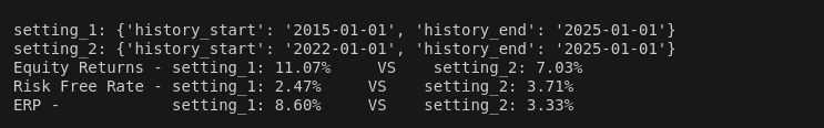
The average equity return and average risk-free rate can be calculated using either a longer historical time period or a shorter historical time period. Both approaches carry advantages and disadvantages. While a longer time period can smooth out noise, a shorter time period is more representative of current market conditions.
| Time Period | Longer | Shorter |
| Advantages | – More reliable with less fluctuating volatility effect | – representative of the current market |
| Disadvantages | – less representative of the current market condition | – increase greater noise due to volatility |
Risk-Free Rate Proxy (Long-Term vs Short-Term)
There is no direct market quote for the risk-free rate. Instead, a proxy is used to represent it, which is typically a government debt instrument, either a long-term government bond or a short-term Treasury bill.

| Risk-Free Proxy | Long-term | Short-term |
| Advantages | – aligning with long-term investment horizons, match the infinite-life of equity | – representative of the current market – suitable for short-term analysis |
| Disadvantages | – missing the short-term market dynamics or changes in monetary policy | – more volatile and less stable over time |
Full Code – Python
import yfinance as yf
import numpy as np

def erp_historical(equity_index, risk_free_proxy, history_start, history_end, mean_type):

    # Step 1: Fetch historical market data of equity index and risk-free rate
    equity_index_close_price = yf.download(equity_index, start=history_start,
                                                    end=history_end)['Close'][equity_index]

    risk_free_rates = yf.download(risk_free_proxy, start=history_start,
                                                    end=history_end)['Close'][risk_free_proxy]

    # Step 2: Calculate annual equity reutrns
    equity_index_return = equity_index_close_price.pct_change()
    if mean_type == 'Geometric':
        equity_index_annual_return = (equity_index_return
                                .resample('Y')
                                .apply(lambda x: (1 + x).prod() - 1)
        )
    else:
        equity_index_annual_return = (equity_index_return
                                .resample('Y')
                                .mean() * 252
        )

    # Step 3: Calculate avarage risk free rate
    risk_free_rate_annual = (risk_free_rates
                                .resample('Y')
                                .mean()/100
    )

    # Step 4: Calculate equity return mean and risk free rate mean
    if mean_type == 'Geometric':
        equity_index_return_mean = (np.prod([1 + r for r in equity_index_annual_return])
                                        ** (1 / len(equity_index_annual_return)) - 1)
        risk_free_rate_mean = (np.prod([1 + r for r in risk_free_rate_annual])
                                        ** (1 / len(risk_free_rate_annual)) - 1)
    else:
        equity_index_return_mean = equity_index_annual_return.mean()
        risk_free_rate_mean = risk_free_rate_annual.mean()

    # Step 5: Compute Equity Risk Premium
    erp = equity_index_return_mean - risk_free_rate_mean

    return erp, equity_index_return_mean, risk_free_rate_mean

def compare_settings(params_1, params_2):

    params = {
        'equity_index': '^GSPC',
        'risk_free_proxy': '^TNX',
        'history_start': '2015-01-01',
        'history_end': '2025-01-01',
        'mean_type': 'Geometric'
    }

    params.update(params_1)
    erp_1, equity_index_mean_1, risk_free_rate_mean_1 = erp_historical(
        equity_index=params['equity_index'],
        risk_free_proxy=params['risk_free_proxy'],
        history_start=params['history_start'],
        history_end=params['history_end'],
        mean_type= params['mean_type']
    )

    params.update(params_2)
    erp_2, equity_index_mean_2, risk_free_rate_mean_2 = erp_historical(
        equity_index=params['equity_index'],
        risk_free_proxy=params['risk_free_proxy'],
        history_start=params['history_start'],
        history_end=params['history_end'],
        mean_type= params['mean_type']
    )

    print('\n')
    print(f"setting_1: {params_1}")
    print(f"setting_2: {params_2}")
    print(f"Equity Returns - setting_1: {equity_index_mean_1 * 100:.2f}%     VS    setting_2: {equity_index_mean_2 * 100:.2f}%")
    print(f"Risk Free Rate - setting_1: {risk_free_rate_mean_1 * 100:.2f}%     VS    setting_2: {risk_free_rate_mean_2 * 100:.2f}%")
    print(f"ERP -            setting_1: {erp_1 * 100:.2f}%     VS    setting_2: {erp_2 * 100:.2f}%")
    print('\n')


erp, equity_index_mean, risk_free_rate_mean = erp_historical(
        equity_index='^GSPC',
        risk_free_proxy='^TNX',
        history_start='2015-01-01',
        history_end='2025-01-01',
        mean_type= 'Geometric'
)
print(f"Average Equity Return: {equity_index_mean * 100:.2f}%")
print(f"Average Risk-Free Rate: {risk_free_rate_mean * 100:.2f}%")
print(f"Equity Risk Premium (ERP): {erp * 100:.2f}%")


# Compare effects of mean type to the ERP
setting_1 = {'mean_type': 'Geometric'}
setting_2 = {'mean_type': 'Arithmetic'}
compare_settings(setting_1, setting_2)

# Compare effects of time periods to the ERP
setting_1 = {'history_start': '2015-01-01', 'history_end': '2025-01-01'}
setting_2 = {'history_start': '2022-01-01', 'history_end': '2025-01-01'}
compare_settings(setting_1, setting_2)

# Compare effects of risk free rate proxy to the ERP
setting_1 = {'risk_free_proxy': '^TNX'}
setting_2 = {'risk_free_proxy': '^IRX'}
compare_settings(setting_1, setting_2)

sublime! Details Emerging About [Future Initiatives/Proposals] 2025 elegant