As discussed in the previous blog post, under the Uncovered Interest Rate Parity condition, the expected change in the exchange rate between two currencies should theoretically offset the interest rate differential between them. This would eliminate any opportunity for investors to profit from interest rate differentials. Fortunately, in the real world, uncovered Interest Rate Parity does not hold over the short and medium term. Empirical studies have shown that high-yield currencies, on average, do not depreciate, and low-yield currencies do not appreciate to the extent predicted by uncovered Interest Rate Parity. This deviation from uncovered Interest Rate Parity creates an opportunity for the FX Carry Trade to emerge as a profitable strategy.

The FX carry trade strategy involves taking long positions in high-yield currencies and short positions in low-yield currencies, profiting from the interest rate differential. I assume the simplest and most intuitive way to explain the carry trade strategy is to walk through a realistic example step by step. In this blog post, I will walk through an FX carry trade case between the Japanese Yen (JPY) and the US Dollar (USD) and present the Python code implemented for this case.

Case Setup

Assume we are able to borrow 1 million Japanese Yen (JPY) at an interest rate of 1% for two years, and the current interest rate for the US Dollar (USD) is 4%. We want to explore the profiting opportunities using a carry trade strategy.

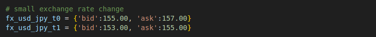
Three exchange rate scenarios will be explored, including a scenario where there is low volatility in the exchange rate.

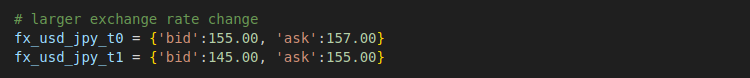
The scenarios where there is high exchange rate volatility.

The scenarios where there are high trade costs, such as a high bid-ask spread.

The second and third scenarios are used to evaluate the effects of high exchange rate volatility and high trade costs, which are two main factors affecting the profitability and risks of carry trades.

Lifecycle of a FX Carry Trade

This is a diagram I created to visualize the entire process of the FX carry trade in our case. This case is based on the first scenario, i.e., low exchange rate volatility.

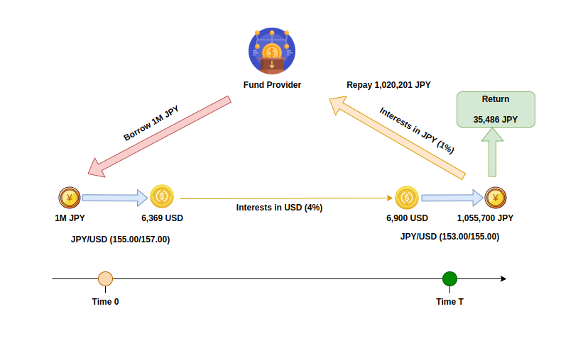
Step 1 – Borrow 1M Japanese Yen for two years at the rate of 1%.

Step 2 – Buy 6,369 USD with the 1M JPY at the quoted ‘ask’ exchange rate at 157.00.

Step 3 – Invest the 6,369 USD into a fixed-income investment with a expected yield at 4%. For the simplicity, we use zero-coupon bond here.

Step 4 – After two years, we have 6,900 USD returned for our USD investment, including both principal and interests.

Step 5 – Buy 1,055,700 JPY back with the 6,900 USD at the quoted ‘bid’ exchange rate of 153.

Step 6 – Repay the 1M JPY along with the 20,201 JPY interests back to the fund provider, and profit the remaining 35,486 JPY.

Code Implementation

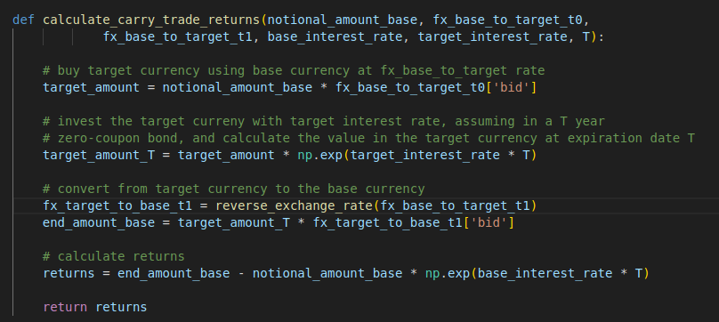
This is the Python code for calculating the carry trade returns based on the given notional amount of the funding currency, the exchange rate between the funding currency and the target currency at time 0 and time T, and the interest rates of both the funding currency and the target currency. The code is straightforward and replicates the carry trade steps described earlier.

Here is the code for calling the function above for the scenario 1. The code for the second and third scenarios is identical, with only the input parameters changing. The full version of the code, including all scenarios, can be found at the bottom of this page.

Here are the results for the three scenarios.

As we can learn from these results, while we can profit from the carry trade in a scenario with low exchange rate volatility, we are at risk of a loss when volatility increases or trading costs are higher.

Full Code – Python

import pandas as pd
import numpy as np

def calculate_carry_trade_returns(notional_amount_base, fx_base_to_target_t0, 
            fx_base_to_target_t1, base_interest_rate, target_interest_rate, T):

    # buy target currency using base currency at fx_base_to_target rate
    target_amount = notional_amount_base * fx_base_to_target_t0['bid']

    # invest the target curreny with target interest rate, assuming in a T year 
    # zero-coupon bond, and calculate the value in the target currency at expiration date T
    target_amount_T = target_amount * np.exp(target_interest_rate * T)

    # convert from target currency to the base currency
    fx_target_to_base_t1 = reverse_exchange_rate(fx_base_to_target_t1)
    end_amount_base = target_amount_T * fx_target_to_base_t1['bid']

    # calculate returns
    returns = end_amount_base - notional_amount_base * np.exp(base_interest_rate * T)
    
    return returns

def reverse_exchange_rate(quote_a_b):
    quote_b_a = {
        'bid': 1 / quote_a_b['ask'],
        'ask': 1 / quote_a_b['bid']
    }

    return quote_b_a


notional_amount_jpy = 1000000
r_usd = 0.04
r_jpy = 0.01
T = 2

# small exchange rate change
fx_usd_jpy_t0 = {'bid':155.00, 'ask':157.00}
fx_usd_jpy_t1 = {'bid':153.00, 'ask':155.00}

returns = calculate_carry_trade_returns(
    notional_amount_base = notional_amount_jpy,
    fx_base_to_target_t0 = reverse_exchange_rate(fx_usd_jpy_t0), 
    fx_base_to_target_t1 = reverse_exchange_rate(fx_usd_jpy_t1),
    base_interest_rate = r_jpy, 
    target_interest_rate = r_usd, 
    T = T
)
print('\n\n')
print(f'Carry trade returns for small fx change: {returns}')

# larger exchange rate change
fx_usd_jpy_t0 = {'bid':155.00, 'ask':157.00}
fx_usd_jpy_t1 = {'bid':145.00, 'ask':155.00}

returns = calculate_carry_trade_returns(
    notional_amount_base = notional_amount_jpy,
    fx_base_to_target_t0 = reverse_exchange_rate(fx_usd_jpy_t0), 
    fx_base_to_target_t1 = reverse_exchange_rate(fx_usd_jpy_t1),
    base_interest_rate = r_jpy, 
    target_interest_rate = r_usd, 
    T = T
)
print(f'Carry trade returns for large fx change: {returns}')

# larger bid-ask spread
fx_usd_jpy_t0 = {'bid':150.00, 'ask':160.00}
fx_usd_jpy_t1 = {'bid':150.00, 'ask':160.00}

returns = calculate_carry_trade_returns(
    notional_amount_base = notional_amount_jpy,
    fx_base_to_target_t0 = reverse_exchange_rate(fx_usd_jpy_t0), 
    fx_base_to_target_t1 = reverse_exchange_rate(fx_usd_jpy_t1),
    base_interest_rate = r_jpy, 
    target_interest_rate = r_usd, 
    T = T
)
print(f'Carry trade returns for large bid-ask spread: {returns}')
print('\n\n')

• Coding towards CFA