
Implied volatility (IV) is a key metric in options trading and risk management. It is derived from the market price of an option and reflects the market’s consensus view on the expected future volatility of the underlying asset.
There is a lot of information that can be interpreted from IV. For example, high IV often signals uncertainty, fear, or the expectation of significant market-moving events, which drives up option prices. Traders can profit by identifying discrepancies between implied volatility and the expected future volatility of the underlying asset.
IV can be calculated using an option pricing model, such as the Black-Scholes Model (BSM), by finding the implied volatility that makes the theoretical price of an option equal to its market price. This process involves solving an equation where the market price of the option is set equal to the option price calculated from the model, with implied volatility as the variable (sigma).
Market Option Price = bsm(S, K, T, r, Sigma)
In this way, the calculation of IV is essentially a root-finding problem to solve the equation. The Newton-Raphson method or the scipy brentq function can be used for root-finding. In this blog post, I will implement the Newton-Raphson method in Python and DolphinDB as examples.
First, we create the function for calculate option price and vega using BSM model.

To calculate the implied volatility, we first provide an initial guess for the IV and use it to calculate the option price and vega with the function we created earlier. We then compare the market option price with the calculated option price based on the guessed IV.

If the difference is smaller than the given threshold, the guessed IV is the right IV we are after. If not, we need to update the sigma guess with the Newton-Raphson formula, and repeat the process.
sigma = sigma – (calculated option price – market option price) / option vega
The full Python code and DolphinDB code can be found at the bottom of this blog post.
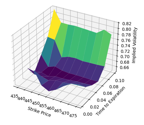
With the function for calculating the IV, we can further generate the volatility surface, which is a 3D visualisation of the market’s expectations for volatility at various strike prices over time.
Full Code – Python
import yfinance as yf
import numpy as np
from scipy.stats import norm
import matplotlib.pyplot as plt
from mpl_toolkits.mplot3d import Axes3D

def calculate_option_vega(s, k, T, r, sigma, option_type="call"):

    # Calculate d1 and d2
    d1 = (np.log(s / k) + (r + 0.5 * sigma ** 2) * T) / (sigma * np.sqrt(T))
    d2 = d1 - sigma * np.sqrt(T)

    # Calculate vega
    option_vega = s * norm.pdf(d1) * np.sqrt(T)

    # Calculate option price
    if option_type == "call":
        option_price = s * norm.cdf(d1) - k * np.exp(-r * T) * norm.cdf(d2)
    else:
        option_price = k * np.exp(-r * T) * norm.cdf(-d2) - s * norm.cdf(-d1)

    return option_vega, option_price

# Resolve implied volatility with Newton-Raphson method
def calculate_implied_volatility(s, k, T, r, marekt_option_price,
        initial_guess=0.2, option_type="call", tolerance=1e-6, iterations=100):

    # Set initial guess
    sigma = initial_guess

    for i in range(iterations):
        print("sigma = "+str(sigma))

        # Calculate the price and vega with current sigma guess
        option_vega, option_price = calculate_option_vega(s, k, T, r, sigma)

        # Difference between the market option price and the
        # option price calculated with the sigma guess
        price_diff = option_price - marekt_option_price

        # return implied volatility when the difference
        # is smaller than the given threshold
        if abs(price_diff) < tolerance:
            return sigma

        # Calculate new sigma using the Newton-Raphson formula
        if option_vega <= 0:
            return None
        else:
            sigma = sigma - price_diff / option_vega

    return None

symbol = 'TSLA'
stock = yf.Ticker(symbol)
expiration_dates = stock.options[:6]
option_chains = {e:stock.option_chain(e) for e in expiration_dates}
TTMs = {e:-(np.datetime64('today', 'D') - np.datetime64(e, 'D')).astype(int) /365
            for e in expiration_dates}
s = stock.history(period="1d")['Close'].iloc[-1]
r = 0.042

strikes = [435, 440, 445, 450, 455.0, 460, 465, 470, 475]
implied_vols = []

for e, option_chain in option_chains.items():

    calls = option_chain.calls
    prices = [calls[calls['strike'] == s]['lastPrice'].iloc[0] for s in strikes]
    ivs = []
    for i in range(len(strikes)):
        iv = calculate_implied_volatility(s, strikes[i], TTMs[e], r, prices[i])
        ivs.append(iv)
    implied_vols.append(ivs)

fig = plt.figure(figsize=(8, 5))
ax = fig.add_subplot(111, projection='3d')
X, Y = np.meshgrid( np.array(strikes), np.array([v for v in TTMs.values()]))

ax.plot_surface(X, Y, np.array(implied_vols), cmap='viridis', edgecolor='none')
ax.set_xlabel('Strike Price')
ax.set_ylabel('Time to Expiration')
ax.set_zlabel('Implied Volatility')
ax.set_title('Option Volatility Surface')
plt.show()
Full Code – DolphinDB
def calculate_option_vega(s, k, T, r, sigma, option_type="call"){

    // Calculate d1 and d2
    d1 = (log(s/k) + (r + 0.5 * pow(sigma,2)) * T) / (sigma * sqrt(T))
    d2 = d1 - sigma * sqrt(T)

    // Calculate vega
    option_vega = s * pdfNormal(0, 1, d1) * sqrt(T)

    // Calculate option price
    if (option_type == "call") {
        option_price = s * cdfNormal(0, 1, d1) - k * exp(-r * T) * cdfNormal(0, 1, d2)
    }
    else {
        option_price = k * exp(-r * T) * cdfNormal(0, 1, -d2) - s * cdfNormal(0, 1, -d1)
    }

    return option_vega, option_price
}

// Resolve implied volatility with Newton-Raphson method
def calculate_implied_volatility(s, k, T, r, marekt_option_price, option_type="call", tolerance=1e-6, iterations=100){

    // Set initial guess
    sigma = 0.2

    for (i in 0:iterations){

        // Calculate the price and vega with current sigma guess
        option_vega, option_price = calculate_option_vega(s, k, T, r, sigma)

        // Difference between the market option price
        // and the option price calculated with the sigma guess
        price_diff = option_price - marekt_option_price

        // return implied volatility when the difference is smaller than the given threshold
        if (abs(price_diff) < tolerance){
            return sigma
        }

        // Calculate new sigma using the Newton-Raphson formula
        if (option_vega <= 0) {
            return NULL
        } else {
            sigma = sigma - price_diff / option_vega
        }
    }

    return NULL
}

s, k, T, r, marekt_option_price = 100, 100, 0.5, 0.05, 4

implied_volatility = calculate_implied_volatility(s, k, r, T, marekt_option_price)
print("Implied Volatility: "+implied_volatility)
