
Options Greeks are key metrics used in options trading and risk management to measure how sensitive an option’s price is a series of factors, including:
- Delta – measures the sensitivity of an option’s price to the changes in the underlying asset’s price.
- Gamma – measures the change rate of an option’s Delta in respect to changes in the underlying asset’s price.
- Theta – measures the sensitivity of an option’s price to the passage of time.
- Vega – measures the sensitivity of an option’s price to changes in the volatility of the underlying asset.
- Rho – measures the sensitivity of an option’s price to changes in interest rates.
Options Greeks can be calculated using a variety of methods, including the Binomial Model, Monte Carlo Simulation, and the Black-Scholes-Merton (BSM) model. For European options, the Black-Scholes-Merton (BSM) model is widely regarded as the simplest and most efficient method for calculating these Greeks. Due to its closed-form formulas and assumptions, the BSM model is a popular choice in both theoretical and practical applications. In this blog, I will explore the calculation and characteristics of options Greek with focus on the BSM model approach.
For options with early exercise, such as American options, or options with changing volatility, the assumptions of the Black-Scholes-Merton (BSM) model no longer hold. In such cases, other models, like the Binomial Model or Monte Carlo Simulation, are required to account for these complexities. I will discuss the Greeks of these options in a separate blog post.
Delta
Delta measures the sensitivity of an option’s price to changes in the price of the underlying asset, i.e., how much the price of an option is expected to change when the price of the underlying asset changes by 1 unit.

To calculate Delta, we differentiate the option price with respect to the underlying asset price, with the option price derived using the BSM formula.

Solving the differentiation gives us the following results. The process of solving the differentiation is not the focus of this blog post, but if you are interested, you can find the full solving steps here.

Here is the Python code implementation.

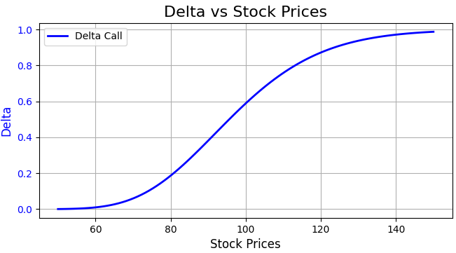
From the formula, we can learn that the delta of a call option ranges from 0 to 1. A larger delta indicates that the option price increases more steeply as the underlying asset price rises. For put options, delta ranges from 0 to -1, meaning the option price moves inversely with the underlying asset price. As shown in the chart below, delta becomes larger as the option moves deeper in-the-money. This means that as the option becomes more in-the-money, the option price changes more rapidly in response to changes in the underlying price. When delta approaches 1, the option price changes dollar-for-dollar with the underlying asset price.
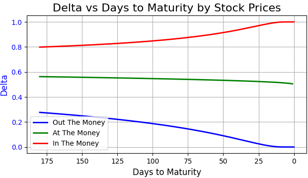
As time progresses toward expiration, delta behaves differently depending on the option’s moneyness. As shown in the chart below, for options that are deep in-the-money, delta moves closer to 1, indicating that the option price closely tracks the underlying asset price. For options that are deep out-of-the-money, delta moves toward 0, meaning the option price becomes less sensitive to changes in the underlying price. When the option is at-the-money, delta remains relatively constant, as small changes in the underlying price have a more balanced effect on the option price.
Gamma
Gamma is the option greek measuring the rate of change of an option’s Delta with respect to changes in the price of the underlying asset, i.e., how much Delta will change when the price of the underlying asset changes by 1 unit. It represents the convexity of the option’s price with respect to the underlying asset’s price. Gamma can be derived by differentiating Delta with respect to the price of the underlying asset.

Solving the differentiation gives us the following results. You can find the full solving steps here.

Here is the Python code implementation.

From the chart, we can see that Gamma is highest at-the-money, indicating that Delta changes most rapidly when the underlying asset price is near the strike price. As the option moves further in or out-of-the-money, Delta becomes less sensitive to changes in the underlying asset’s price.

Theta
Theta measures the sensitivity of the option’s price to the passage of time, i.e., how much the price of an option will change as time passes. Theta can be derived by differentiating option price with respect to time to maturity.

Solving the differentiation gives us the following results. You can find the full solving steps here.

Here is the Python code implementation.

From the formula above, we can see that Theta will always be negative for both call and put options, reflecting the time decay of the option’s price. Theta impacts the option price based on its moneyness. At-the-money options typically have a larger negative Theta than deep in-the-money or out-of-the-money options. Additionally, Theta becomes more negative as the option approaches expiration, accelerating the time decay.
Vega
Vega measures the sensitivity of the option’s price to changes in volatility, i.e., how much the price of an option will change for one unit change in volatility. Vega can be derived by differentiating option price with respect to volatility.

Solving the differentiation gives us the following results. You can find the full solving steps here.

Here is the Python code implementation.

Vega is typically positive for both call and put options, meaning that an increase in the volatility of the underlying asset makes the option more expensive, regardless of whether it’s a call or put. This is understandable because higher volatility increases the potential for larger price swings, which raises the risk. To offset this additional risk, the cost of the option increases. In addition, Delta and Gamma are also influenced by volatility. As volatility increases, the option price becomes more sensitive to changes in the underlying asset’s price, leading to greater fluctuations in Delta and Gamma.

On the other side, Vega can be affected by both moneyness and time decay. As shown in the chart below, Vega tends to be higher when the option is at-the-money. Additionally, due to the higher uncertainty associated with options near expiration, Vega typically decreases as time to expiration shortens.

Rho
Rho measures the sensitivity of an option’s price to changes in the risk-free interest rate, i.e., how much the price of an option will change for one unit change in interest rate. Rho can be derived by differentiating option price with the interest rate.

Solving the differentiation gives us the following results. You can find the full solving steps here.

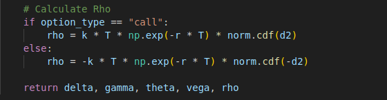
Here is the Python code implementation.
As the chart below shows, Rho is typically positive for call options, meaning that the price of a call option increases when interest rates rise. On the other hand, for put options, the option price is inversely related to interest rates, meaning that as interest rates increase, the price of the put option decreases.

Full Code – Python
import numpy as np
from scipy.stats import norm
import matplotlib.pyplot as plt

def calculate_d1_d2(s, k, T, r, sigma):
    d1 = (
            (np.log(s/k) + (r + 0.5 * sigma ** 2) * T)
                / (sigma * np.sqrt(T))
    )
    d2 = d1 - sigma * np.sqrt(T)

    return d1, d2

def calculate_greeks(s, k, T, r, sigma, option_type="call"):

    d1, d2 = calculate_d1_d2(s, k, T, r, sigma)

    # Calculate Delta
    if option_type == "call":
        delta = norm.cdf(d1)
    else:
        delta = norm.cdf(d1) - 1

    # Calculate Gamma
    gamma = norm.pdf(d1) / (s * sigma * np.sqrt(T))

    # Calculate Theta
    if option_type == "call":
        theta = (-s * norm.pdf(d1) * sigma / (2 * np.sqrt(T))
                 - r * k * np.exp(-r * T) * norm.cdf(d2))
    else:
        theta = (-s * norm.pdf(d1) * sigma / (2 * np.sqrt(T))
                 + r * k * np.exp(-r * T) * norm.cdf(-d2))

    # Calculate Vega
    vega = s * norm.pdf(d1) * np.sqrt(T)

    # Calculate Rho
    if option_type == "call":
        rho = k * T * np.exp(-r * T) * norm.cdf(d2)
    else:
        rho = -k * T * np.exp(-r * T) * norm.cdf(-d2)

    return delta, gamma, theta, vega, rho

def calculate_option_value(s, k, T, r, sigma, option_type="call"):

    # Calculate d1 and d2
    d1, d2 = calculate_d1_d2(s, k, T, r, sigma)

    # Calculate option price
    if option_type == "call":
        option_price = s * norm.cdf(d1) - k * np.exp(-r * T) * norm.cdf(d2)
    else:
        option_price = k * np.exp(-r * T) * norm.cdf(-d2) - s * norm.cdf(-d1)

    return option_price


def draw_chart(title, x_data, x_title, y1, y1_title, y2_data=None, y2_title=None, x_invert=False):

    fig, ax1 = plt.subplots(figsize=(8, 4))

    for y in y1:
        ax1.plot(x_data, y[0], label=y[1], color=y[2], linewidth=2)
    ax1.set_xlabel(x_title, fontsize=12)
    ax1.set_ylabel(y1_title, color='b', fontsize=12)
    ax1.tick_params(axis='y', labelcolor='b')
    ax1.grid(True)

    if y2_data is not None:
        ax2 = ax1.twinx()
        ax2.plot(x_data, y2_data, label=y2_title, color='red', linewidth=2)
        ax2.set_ylabel(y2_title, color='red', fontsize=12)
        ax2.tick_params(axis='y', labelcolor='red')

    if x_invert:
        ax=plt.gca()
        ax.invert_xaxis()
    plt.legend()
    plt.title(title, fontsize=16)
    fig.tight_layout()
    plt.show()


s, k, T, r, sigma = 100, 100, 1, 0.025, 0.2
stock_prices = np.linspace(50, 150, 100)
delta_c, gamma_c, theta_c, vega_c, rho_c  = [], [], [], [], []
for s in stock_prices:
    g_d, g_g, g_t, g_v, g_r = calculate_greeks(s, k, T, r, sigma, "call")
    delta_c.append(g_d)
    gamma_c.append(g_g)
    theta_c.append(g_t)
    vega_c.append(g_v)
    rho_c.append(g_r)


#draw chart Delta vs Stock Prices
draw_chart("Delta vs Stock Prices", stock_prices, "Stock Prices",
           [(delta_c, "Delta Call", "b")], "Delta")

#draw chart Delta vs Gamma
draw_chart("Delta vs Gamma", stock_prices, "Stock Prices",
            [(delta_c, "Delta Call", "b")], "Delta", gamma_c, "Gamma")


#draw chart Delta vs Days to Maturity
valuing_prices = [90, 100, 110]
dtm = np.linspace(0, 180, 180)
price_delta, delta_c = [], []
for s in valuing_prices:
    for t in dtm:
        g_d, g_g, g_t, g_v, g_r = calculate_greeks(s, k, t/365, r, sigma, "call")
        delta_c.append(g_d)

    price_delta.append(delta_c)
    delta_c = []

draw_chart("Delta vs Days to Maturity by Stock Prices", dtm, "Days to Maturity",
           [(price_delta[0], "Out The Money", "b"),
            (price_delta[1], "At The Money", "g"),
            (price_delta[2], "In The Money", "red"),
            ], "Delta", x_invert=True)


#draw chart Vega vs Days to Maturity
dtm=[10, 20, 30]
dtm_vega, vega_c =[], []
for t in dtm:
    for s in stock_prices:
        g_d, g_g, g_t, g_v, g_r = calculate_greeks(s, k, t/365, r, sigma, "call")
        vega_c.append(g_v)

    dtm_vega.append(vega_c)
    vega_c = []

draw_chart("Vega vs Stock Prices by Days to Maturity", stock_prices, "Stock Prices",
           [(dtm_vega[0], "10 Days to Maturity", "b"),
            (dtm_vega[1], "20 Days to Maturity", "g"),
            (dtm_vega[2], "30 Days to Maturity", "red"),
            ], "Vega")


#draw chart option prices vs volatility
s, k, T, r, sigma = 100, 100, 1, 0.025, 0.2
sigmas = np.linspace(0, 30, 30)
option_prices_call, option_prices_put = [], []
for v in sigmas:
    option_prices_call.append(calculate_option_value(s, k, T, r, v/100, "call"))
    option_prices_put.append(calculate_option_value(s, k, T, r, v/100, "put"))

draw_chart("Volatility vs options prices", sigmas/100, "Volatility",
           [(option_prices_call, "Call Option", "b"),
            (option_prices_put, "Put Option", "g")
            ], "Option Price")


#draw chart option prices vs interest rates
s, k, T, r, sigma = 100, 100, 1, 0.025, 0.2
rates = np.linspace(0, 10, 100)
option_prices_call, option_prices_put = [], []
for rate in rates:
    option_prices_call.append(calculate_option_value(s, k, T, rate/100, sigma, "call"))
    option_prices_put.append(calculate_option_value(s, k, T, rate/100, sigma, "put"))

draw_chart("Interest rates vs options prices", rates/100, "Interest rate",
           [(option_prices_call, "Call Option", "b"),
            (option_prices_put, "Put Option", "g")
            ], "Option Price")
Full Code – DolphinDB
def calculate_d1_d2(s, k, T, r, sigma){

    d1 = (log(s/k)+(r+0.5*pow(sigma,2))*T) / (sigma*sqrt(T))

    d2 = d1-sigma*sqrt(T)

    return d1, d2
}

def calculate_greeks(s, k, T, r, sigma, option_type="call"){

    // calculate d1, d2
    d1, d2 = calculate_d1_d2(s, k, T, r, sigma)

    // calculate Delta
    if (option_type == "call")
        delta = cdfNormal(0, 1, d1)
    else
        delta = cdfNormal(0, 1, d1) - 1

    // calculate Gamma
    gamma = pdfNormal(0, 1, d1) / (s*sigma*sqrt(T))

    // calculate Theta
    if (option_type == "call")
        theta = (-s * pdfNormal(0, 1, d1)*sigma / (2*sqrt(T)) - r*k*exp(-r*T)*cdfNormal(0, 1, d2))
    else
        theta = (-s * pdfNormal(0, 1, d1)*sigma / (2*sqrt(T)) + r*k*exp(-r*T)*cdfNormal(0, 1, -d2))

    // calculate Vega
    vega = s * pdfNormal(0, 1, d1) * sqrt(T)

    // calculate Rho
    if (option_type == "call")
        rho = k * T * exp(-r * T) * cdfNormal(0, 1, d2)
    else
        rho = -k * T * exp(-r * T) * cdfNormal(0, 1, -d2)

    return delta, gamma, theta, vega, rho
}

s, k, T, r, sigma = 100, 100, 1, 0.025, 0.2
delta, gamma, theta, vega, rho = calculate_greeks(s, k, T, r, sigma)
print("Delta is "+delta)
print("Gamma is "+gamma)
print("Theta is "+theta)
print("Vega is "+vega)
print("Rho is "+rho)
