
In the previous article, I discussed Contractual Definition for InterestRatePayout — the accrual periods, payment dates, reset dates, stubs, day count convention, and compounding method that turn an economic agreement into a precise contractual structure.
Those attributes are essential. But they still do not give us a payment amount. They tell us what the contract says. They do not yet tell us what value should be paid for a specific period.
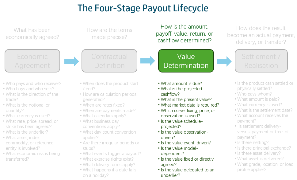
This article moves to the next F-PAL stage: Value Determination. The main question for this stage is: how do the contractual terms become calculated amounts?
For an interest rate payout, this is where dates, notional, rate logic, fixings, observations, spreads, day count fractions, compounding, and discounting come together to determine a value. In a traditional system, this logic may be hidden inside a pricing engine. In an AI-native financial data foundation, we want the calculation path to be explicit enough for a system, a human, or an AI agent to explain.
CalculationPeriod — The Working Unit
Interest is not calculated at the whole-trade level. It is calculated period by period. At the contractual level, CalculationPeriodDates tells us how periods should be generated. At the value determination level, we need the actual generated period: start date, end date, number of days, year fraction, notional in effect, rate in effect, and calculated amount.
In CDM calculation logic, this generated period is represented through CalculationPeriodData. Conceptually, this is the working unit for calculation.
For example:
CalculationPeriodDates- effectiveDate = 15 Mar 2026- firstRegularPeriodStartDate = 30 Jun 2026- calculationPeriodFrequency = 6M- terminationDate = 30 Jun 2029- stubPeriodType = ShortInitial
The first generated CalculationPeriod is:
CalculationPeriod- adjustedStartDate = 16 Mar 2026- adjustedEndDate = 30 Jun 2026- calculationPeriodNumberOfDays = 106- notionalAmount = 100000000- fixedRate = 0.035- dayCountYearFraction = 0.29444- forecastAmount = USD 1,030,556
This generated period becomes the working unit for calculation. Interest is not calculated at the whole-trade level. It is calculated period by period. CalculationPeriod is the bridge between Contractual Definition and Value Determination — it holds the period dates, the notional, the rate, the derived day count fraction, and the resulting forecast amount all in one place.
With the container established, the next question is: for a given period, what rate value is actually used? The contract may say “3M SOFR + 25bp”, but that is a rule, not a number. We need to trace how the rule becomes a number before we can combine it with anything else.
Where Does the Rate Come From?
From Rule to Observation
The distinction between rate specification and rate observation is one of the most important modelling separations in the CDM. These are three different types at three different levels:
FloatingRateSpecification ← what the contract says rateOption: SOFR indexTenor: 6M spreadSchedule: +25bp capRateSchedule: 6.00% floorRateSchedule: 0.00% initialRate: (empty — not yet known for future periods) finalRateRounding: 5 decimal places averagingMethod: Unweighted negativeInterestRateTreatment: ZeroFloor ↓ for a specific period, it becomes:FloatingRateDefinition ← what happened for one period calculatedRate: 0.0545 (5.45% = 5.20% + 0.25%) floatingRateMultiplier: 1.0 rateObservation: [ ← the actual fixings that fed in RateObservation { observationDate: 2026-06-26 observedRate: 0.0520 adjustedFixingDate: 2026-06-26 } ]
FloatingRateDefinition carries calculatedRate, rateObservation (0..*), and floatingRateMultiplier. Each RateObservation carries observationDate, observedRate, and adjustedFixingDate.
This allows the model to answer two different questions: what was the contractual rate rule? and what rate value was actually used for this period? If we only store the observed rate, we lose the contractual explanation. If we only store the contractual rule, we cannot explain the calculated amount.
Known or Projected?
Once we have the observation structure, the next question is the status of each observation. A past period may have a known fixing. A future period may require a projected forward rate. An in-progress overnight period may be partially known and partially projected.
A cashflow amount based on a known fixing should not be treated in the same way as one based on a projected rate. An AI agent should be able to say: this amount is known because the fixing has already occurred, or this amount is projected because the fixing date is in the future.
One Fixing or Many?
In the simple term-rate case, the reset frequency is once per calculation period. One fixing determines the rate for the whole period. But for overnight indexed payouts, the rate may be observed daily within a quarterly period.
The CDM keeps three frequencies separate because they live on three different types:
| Frequency | CDM Type | Attribute |
|---|---|---|
| Accrual rhythm | CalculationPeriodDates | calculationPeriodFrequency |
| Reset/observation rhythm | ResetDates | resetFrequency |
| Payment rhythm | PaymentDates | paymentFrequency (implied by schedule) |
These do not have to be the same. A quarterly accrual period may contain daily resets and quarterly payments. The CDM structure prevents collapsing all three into one schedule.
Now we have the rate. The contract told us the rule; the observation gave us the number; the frequency told us how many observations apply. The next step is to combine the rate with notional, time, and adjustments to produce an amount.
From Rate to Amount
The Simplest Case: Fixed Rate
No observations. No projections. No compounding. Just notional, rate, and time.
At the contract level: notional = USD 100,000,000, fixed rate = 3.50%, day count fraction = ACT/360, calculation period = 16 Mar 2026 to 30 Jun 2026.
Fixed Amount = Notional × Fixed Rate × Day Count Fraction = USD 100,000,000 × 3.50% × 106 / 360 = USD 1,030,556
In the CDM, the computed result is captured by FixedAmountCalculationDetails:
type FixedAmountCalculationDetails: calculationPeriod CalculationPeriodBase (1..1) calculationPeriodNotionalAmount Money (1..1) fixedRate number (1..1) yearFraction number (1..1) calculatedAmount number (1..1)
This type carries the full input-to-output trace: which period, what notional, what fixed rate, what year fraction, what amount.
Applying What We Learned: Floating Rate
Now the rate comes from an observation rather than a stored number, and adjustments may apply.
Floating Amount = Notional × Adjusted Floating Rate × Day Count Fraction
Where the adjusted floating rate may include: observed rate (5.20%), plus spread (0.25%), subject to cap and floor, subject to rounding, subject to compounding or averaging.
For the period 30 Jun 2026 to 31 Dec 2026, with 3M SOFR fixing at 5.12% on 28 Jun 2026:
USD 100,000,000 × 5.12% × 184 / 360 = USD 2,616,889
The separation established earlier — FloatingRateSpecification for the rule, FloatingRateDefinition for the period result, RateObservation for the individual fixings — means the model can explain not just the final amount but every step that produced it.
Day Count: Time into Numbers
Day count looks like a small field, but it directly affects the calculated amount. The same start and end dates produce different year fractions under ACT/360 versus 30/360 versus ACT/ACT.
In the CDM, day count operates at two levels. At the contract level, dayCountFraction (DayCountFractionEnum) sits directly on InterestRatePayout — it says “use ACT/360.” At the period level, the derived result is dayCountYearFraction on CalculationPeriod — it says “106 / 360 = 0.29444” for one period or “184 / 360 = 0.51111” for another. A model that wants to explain an amount needs both.
Compounding and Averaging: Many Observations into One Rate
For a simple term-rate payout, one fixing produces one rate. But for overnight indexed rates, the final period rate is derived from many daily observations. In the CDM, these details live in FloatingRateCalculationParameters, on the FloatingRate type:
type FloatingRateCalculationParameters: calculationMethod FloatingRateCalculationMethodEnum dayCountBasis DayCountFractionEnum lockoutPeriod LockoutPeriod (0..1) lookbackPeriod LookbackPeriod (0..1) observationShift ObservationShift (0..1)
The calculated rate may be the result of a process over many observations. If the model only stores the final rate, the AI can repeat the result but cannot explain it. If the model preserves the relationship between period, observations, compounding method, and resulting rate, the AI can explain how the value was produced.
Discounting: Adjusting for Payment Timing
Some products discount the calculated amount because payment occurs at the beginning of the period rather than at the end — most commonly FRAs.
In the CDM, this is discountingMethod (DiscountingMethod, product-asset-type.rosetta):
type DiscountingMethod: discountingType DiscountingTypeEnum (1..1) // Standard, FRA, FRAYield discountRate number (0..1) discountRateDayCountFraction DayCountFractionEnum (0..1)
This is contractual discounting — an adjustment to the calculated amount based on settlement timing — not to be confused with valuation discounting of all future cashflows.
Spread Calculation Method: A Narrower Case
For asset swaps, the spread calculation method — spreadCalculationMethod (SpreadCalculationMethodEnum, with values ParPar and Proceeds) on InterestRatePayout — affects how the spread is determined. The principle is the same one that runs through all four stages: do not hide financial meaning inside a number. Represent the method where the method matters.
The Full Chain: One IRS, One Period
We have now seen each piece individually. The final step is to connect them. Here, we use an assuming example to present the full chain.
A USD 100M fixed-float IRS. Party A pays fixed 4.00% semi-annual, receives 3M SOFR quarterly. The period shown is 30 Jun 2026 to 31 Dec 2026. For the floating leg, 3M SOFR fixed at 5.12% on 28 Jun 2026.
Derived Value Lineage
Some values in this chain are inputs. Others are outputs. In the CDM, the fixedAmount and floatingAmount attributes on InterestRatePayout are typed with the Rosetta calculation keyword — a type-level signal that these are computed, not stored.
Tracing backwards from either gives the full lineage:
fixedAmount ← notional (from ResolvablePriceQuantity) ← fixed rate (from FixedRateSpecification) ← day count fraction (from dayCountFraction, applied to the period) ← calculation period (from CalculationPeriod)floatingAmount ← notional (from ResolvablePriceQuantity) ← observed rate (from RateObservation) ← spread (from FloatingRateBase) ← cap / floor (from FloatingRateBase) ← compounding method (from compoundingMethod / FloatingRateCalculationParameters) ← day count fraction (from dayCountFraction, applied to the period) ← calculation period (from CalculationPeriod)
This lineage is what makes the amount explainable. It is also what makes it debuggable, reconcilable, and auditable.
What This Means for AI-Native Financial Data
Value Determination is where an AI-native financial data foundation becomes more than a semantic dictionary.
It is not enough for the model to know what “notional,” “SOFR,” “spread,” and “day count” mean. The model must also know how they interact to produce an amount. This is where semantic modelling meets executable calculation.
For AI agents, the value is not that they can guess a formula. The value is that they can inspect structured inputs, follow calculation lineage, and explain the result:
- This is a floating interest amount.
- It is calculated for the period from 30 Jun 2026 to 31 Dec 2026.
- The notional is USD 100 million.
- The rate is 3M SOFR observed on 28 Jun 2026 at 5.12%.
- The day count convention is ACT/360, giving a year fraction of 0.51111.
- No compounding, no discounting, no cap or floor applies.
- Therefore this period produces a floating amount of USD 2,616,889.
That is grounded reasoning over financial structure — a very different capability from simply generating text about swaps.
Conclusion
Economic Agreement tells us what the parties agreed. Contractual Definition tells us how that agreement is written into dates, schedules, resets, stubs, day count, and compounding terms. Value Determination tells us how those terms become calculated amounts.
This article traced that path through three questions, answered in sequence: where does the calculation happen? (CalculationPeriod), where does the rate come from? (specification → observation → known/projected → frequency), and how does the rate become an amount? (fixed → floating → day count → compounding → discounting → spread). The synthesis section brought all the pieces together in a single calculation chain, with derived value lineage to keep it coherent.
The next article covers Settlement / Realisation — where the calculated amount becomes a settled cashflow, a principal exchange, or a projected obligation.
