In the previous article, I discussed the first F-PAL stage for InterestRatePayout: Economic Agreement. Economic Agreement tells us what has been commercially agreed: who pays, who receives, what notional applies, and what rate logic determines the obligation.

But an interest rate payout cannot be understood from economic terms alone. Instead, interest is always connected to time.

• A rate applies over a period.
• An amount accrues over a period.
• A floating rate may reset or fix on a specific date.
• The resulting cash amount is paid on a payment date.
• Irregular first or last periods may need special treatment.

This is why the second F-PAL stage is necessary: Contractual Timing.

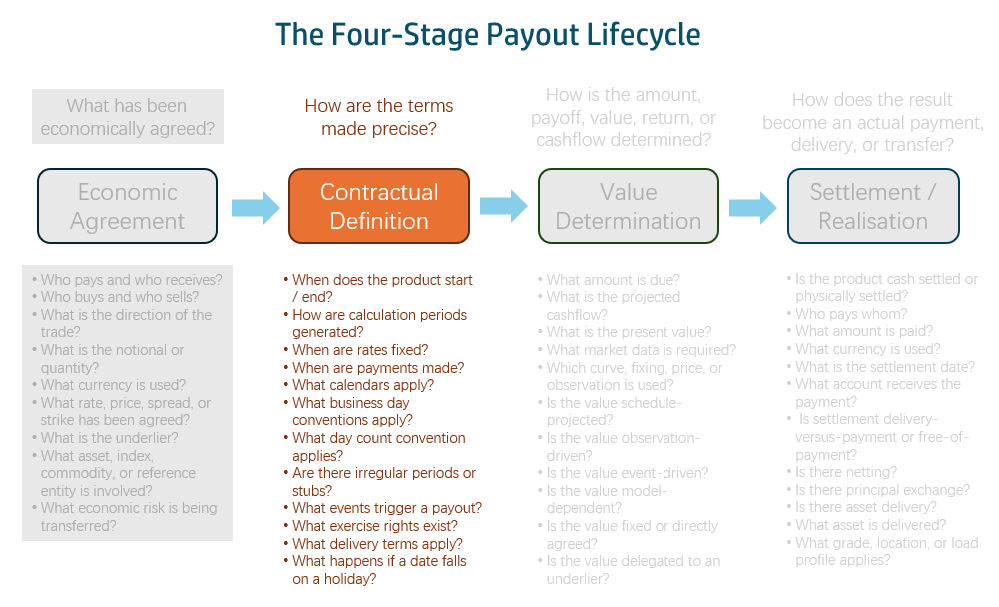
Contractual Timing answers the question: How is the economic agreement organised through time? For InterestRatePayout, this mainly means the time structure of the payout.

The model needs to define:

• when interest accrues;
• when cash is paid;
• when rates reset or fix;
• how irregular periods are handled.

A common mistake in financial data modelling is to collapse time into one or two date fields: start date, end date, maturity date, maybe payment date. That is not enough. Interest rate products depend on several different kinds of dates, and each date has a different business meaning.

The accrual period defines the period over which interest is earned or owed.

The payment date defines when the resulting cash is actually paid.

The reset or fixing date defines when a floating rate is observed or determined.

The stub period defines how irregular first or last periods are treated.

A good canonical model keeps these concepts separate. That separation is not unnecessary complexity. It is the contractual timing of the economic agreement.

1. Accrual — Over What Period Does Interest Accrue?

The first part of Contractual Timing is accrual.

An interest amount is not just based on notional and rate. It is based on notional and rate over a period of time. For example, a fixed coupon may accrue from 1 January to 31 March. A floating coupon may accrue from one reset period to the next. An overnight compounded payout may accrue over a period containing many daily observations. The accrual period defines the economic period to which the interest amount relates.

This is different from the payment date.

A payment may be made after the accrual period ends. For example, interest may accrue from 1 January to 31 March, but the cash may be paid on 2 April or 5 April depending on business day adjustments.

In the CDM, this contractual structure is represented through CalculationPeriodDates. The type defines two things at the same time: the overall envelope of the payout and the rhythm inside that envelope.

The envelope is defined by effectiveDate and terminationDate.

The rhythm is defined by calculationPeriodFrequency, roll convention, and related date adjustment rules.

The type also carries calculationPeriodDatesAdjustments, which defines the business day convention and financial centres that govern how period boundaries adjust when they fall on non-business days. This is important because financial contracts do not operate on abstract calendar dates only. They operate through market calendars, business day conventions, and financial centre rules.

CalculationPeriodDates {
    effectiveDate: AdjustableOrRelativeDate {
        adjustableDate: AdjustableDate {
            unadjustedDate: 2026-03-15
        }
    }
    terminationDate: AdjustableOrRelativeDate {
        adjustableDate: AdjustableDate {
            unadjustedDate: 2029-06-15
        }
    }
    calculationPeriodFrequency: CalculationPeriodFrequency {
        period: 6M
        periodMultiplier: 1
        rollConvention: 15
    }
    calculationPeriodDatesAdjustments: BusinessDayAdjustments {
        businessDayConvention: ModifiedFollowing
        businessCenters: BusinessCenters { businessCenter: EUTA }
    }
    firstPeriodStartDate: AdjustableOrRelativeDate {
        adjustableDate: AdjustableDate { unadjustedDate: 2026-03-15 }
    }
    firstRegularPeriodStartDate: 2026-06-15
    stubPeriodType: [ ShortInitial ]
}

The CDM also provides explicit treatment for edge cases: firstPeriodStartDate, firstRegularPeriodStartDate, lastRegularPeriodEndDate, and stubPeriodType. These attributes allow the model to represent schedules that do not fit a perfectly regular pattern.

The modelling point is simple: the accrual schedule is not just a pair of dates. It is a contractual structure.

For AI-native financial data, this matters because an AI agent should be able to understand that a payout is not merely “3M SOFR”. It should also understand what the three-month periods are, how they are generated, and how they align with payment and reset logic.

2. Payment Timing — When Is Cash Expected to Be Exchanged?

The second part of Contractual Timing is payment timing.

Payment is not the same as accrual. Interest may accrue to 31 March but be paid on 2 April. Another product may pay two business days after the period end. Another may pay on a single bullet date. Another may have a delayed payment feature.

The payment structure answers the question: When is the cash expected to be exchanged?

The CDM captures this separation through a deliberate structural choice. An InterestRatePayout can use either a recurring payment date structure or a single payment date structure.

A recurring-payment product, such as a swap or floating-rate note, uses PaymentDates. This can include schedule parameters such as firstPaymentDate, lastRegularPaymentDate, paymentDaysOffset, and paymentDatesAdjustments.

paymentDates: PaymentDates {
    firstPaymentDate: 2026-06-17
    lastRegularPaymentDate: 2029-06-17
    paymentDaysOffset: Offset {
        period: D
        periodMultiplier: 2
    }
    paymentDatesAdjustments: BusinessDayAdjustments {
        businessDayConvention: ModifiedFollowing
        businessCenters: BusinessCenters { businessCenter: USNY }
    }
}

A single-payment product, such as an FRA or zero-coupon structure, may use a single adjustable payment date instead.

This is not a minor field definition. It is a type-level assertion that a payout with a recurring payment schedule and a payout with a single bullet payment are structurally different, even though both may be InterestRatePayouts.

For AI-native financial data, this matters because payment timing affects cashflow projection, liquidity, settlement, reconciliation, and reporting. If an AI agent is asked what cash is due next month, it cannot answer from accrual dates alone. It needs payment dates. If it is asked whether a payout is a recurring coupon stream or a single settlement amount, it needs to understand the payment structure.

That is why payment timing belongs to Contractual Timing.

However, this is only the contractual rule for payment timing. The actual projected payment amount is not created yet. That belongs to the next stage: Value Determination.

3. Fixing — When Is the Rate Determined?

The third part of Contractual Timing is fixing or reset behaviour. This is mainly relevant for floating-rate payouts.

A floating-rate payout usually does not know its final rate at trade inception. The rate must be observed, fixed, or determined according to contractual rules.

For example, a 3M SOFR payout may reset at the start of each calculation period. An overnight indexed payout may involve daily observations throughout the accrual period. A rate may be fixed two business days before the start of the period. Another rate may use lookback, lockout, observation shift, or rate cut-off rules.

The reset structure answers the question: when and how is the rate determined?

This is separate from both accrual and payment. A payout may accrue from January to March. The rate may be fixed before the period starts. The payment may be made after the period ends. These are three different date concepts, and they carry different business meanings.

In the CDM, this is represented through ResetDates. The type separates several concerns: whether reset occurs relative to the start or end of the calculation period, how frequently the rate resets, what fixing dates apply, how the initial fixing date is handled, and what business day adjustments govern those dates.

ResetDates {
    calculationPeriodDatesReference: CalculationPeriodDates {          // → points to the accrual schedule
        reference: "floating-leg-calculation-period-dates"
    }
    resetRelativeTo: CalculationPeriodStartDate
    resetFrequency: ResetFrequency {
        period: 3M
        periodMultiplier: 1
    }
    fixingDates: AdjustableRelativeOrPeriodicDates {
        period: 3M
        periodMultiplier: 1
        businessDayConvention: Preceding
        businessCenters: BusinessCenters { businessCenter: USNY }
        offset: Offset {
            period: D
            periodMultiplier: -2            // 2 business days BEFORE period start
        }
    }
    initialFixingDate: InitialFixingDate {
        adjustableDate: AdjustableDate {
            unadjustedDate: 2026-03-11
        }
    }
    resetDatesAdjustments: BusinessDayAdjustments {
        businessDayConvention: Preceding
        businessCenters: BusinessCenters { businessCenter: USNY }
    }
}

In this example, the reset schedule says three things:

• When does the rate apply? At the start of each calculation period, not the end. That is what resetRelativeTo: CalculationPeriodStartDate means. For a rate set in arrears, this would be CalculationPeriodEndDate instead.
• How often does it reset? Once per quarterly period. The resetFrequency matches the accrual rhythm — one reset per period, observed 2 business days before it begins. For an overnight-indexed payout, this would be daily instead.
• How is the fixing date determined? By counting backwards 2 business days from the period start, using the Preceding convention and the USNY calendar. The initialFixingDate handles the very first fixing, which may already be known at trade inception.

The reset schedule is also semantically connected to the accrual schedule. A reset date is not just an arbitrary date. It is usually defined relative to the calculation period. That relationship is important. If reset dates are separated from accrual periods without reference, the model loses meaning. The fixing schedule should be understood in relation to the periods whose rates it determines.

For AI-native financial data, if an AI agent wants to explain a floating payout, it needs to know not only the floating index but also the fixing logic.

The following diagram shows the temporal events relation in a single period.

4. Stubs — How Are Irregular Periods Handled?

The fourth part of Contractual Timing is stub treatment.

Most trades do not always start and end on perfect schedule boundaries. A trade may start on 15 March even though regular quarterly periods would normally run from quarter-end to quarter-end. The first period may therefore be short or long. The final period may also be irregular.

These irregular periods are called stubs. Stub periods matter because they can affect rate determination, accrual calculation, interpolation, and payment amount.

For example, if a swap has a short first coupon period, the rate may still be based on a standard tenor, or it may be interpolated between two tenors. If the final period is longer than usual, special treatment may be required.

This is why stub logic should not be hidden in free text or ignored as an exception. CalculationPeriodDates captures the irregular timing through fields such as firstRegularPeriodStartDate, lastRegularPeriodEndDate, and stubPeriodType. StubPeriod is only needed when the irregular period has special economic treatment, such as interpolation, a different tenor, an agreed stub rate, or an agreed stub amount. It can specify an initialStub or finalStub, each represented through StubValue.

A StubValue can represent several different treatments. It may specify one or two floating rate tenors. One tenor means that a different tenor is used for the stub. Two tenors can support interpolation between tenors. Alternatively, the stub may use an explicitly agreed stubRate or an explicitly agreed stubAmount.

StubPeriod {
    calculationPeriodDatesReference: CalculationPeriodDates {
        reference: "floating-leg-calculation-period-dates"
    }
    initialStub: StubValue {
        floatingRate: [
            StubFloatingRate {
                floatingRateIndex: EURIBOR
                indexTenor: 3M
            },
            StubFloatingRate {
                floatingRateIndex: EURIBOR
                indexTenor: 6M
            }
        ]
    }
}

This is structural parsimony. The model does not force unnecessary detail into the common case. If the irregularity is already captured by the calculation period dates and nothing special happens economically, extra stub detail may not be needed. But when the stub has special economic treatment, the model provides a place to represent it.

A model that can expose stubs explicitly gives both humans and AI agents a better chance of understanding and validating the trade.

Boundary Attributes: Day Count and Compounding

Some attributes sit at the boundary between Contractual Timing and the next F-PAL area, Value Determination.

Two important examples are dayCountFraction and compoundingMethod.

The day count fraction is contractually defined, but it becomes operational during calculation. It tells the model how to convert a period of time into a year fraction. For example, the same 90-day period may produce a different accrual fraction under ACT/360, 30/360, or ACT/ACT. The interest amount therefore depends not only on notional and rate, but also on the contractual day count convention. This is not a minor technical detail. In interest rate products, day count convention is part of the economics.

Compounding method is similar. It is specified as part of the contract, but it becomes meaningful when determining the payment amount. If calculation periods and payment periods differ, multiple calculation periods may contribute to one payment. In that case, the compounding method tells the system how those period amounts interact. For example, an overnight indexed payout may require compounded daily rates. Another structure may use no compounding. Another may require a specific spread treatment.

These attributes show why F-PAL areas are connected rather than isolated.

Contractual Timing provides the rules. Value Determination uses those rules to calculate amounts.

Final Thought

Contractual Timing is the second layer of understanding InterestRatePayout.

Economic Agreement defines the core commercial obligation: who pays, who receives, what notional applies, and what rate logic determines the payout.

Contractual Timing turns that agreement into precise contractual time structure: when interest accrues, when cash is expected to be paid, when rates reset or fix, and how irregular periods are handled.

Together, these two stages turn InterestRatePayout from a vague interest payment idea into a structured financial component. But the payout still has not been calculated. At this point, the model knows the obligation and the timing rules. It does not yet know the calculated amount for each period.

That is the role of the next F-PAL stage: Value Determination.

In the next article, I will continue the analysis with CalculationPeriod, FloatingRateDefinition, and FixedAmountCalculationDetails. That is where the payout moves from contractual timing to calculated amounts and projected payment values.

• *AI-Native Financial Data Foundation